
Fitting Observed Spectra to Models
Overview: Students fit both visible light spectra (manually, using Spectrum Explorer and slider bars for model parameters) and X-ray spectra (by computer, using CIAO / Sherpa spectral fitting engine, with automatic determination of best fit parameters for each model). Students then discuss what constitutes a "good fit."
Physical resources: None
Electronic resources: Chandra images of RBS1223 (obsid 731) and M81 (obsid 5943).
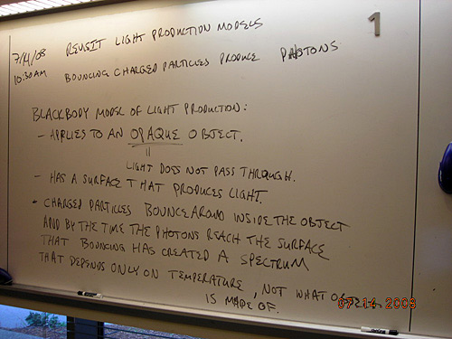
Revisit production mechanisms of light from "bouncing charged particles," and corresponding models.
- Blackbody spectrum model: for an opaque (you can't see through it) object. Charged particles bounce around inside the object, and by the time the photons reach the surface, that bouncing has created a distribution of light that is the same, regardless of what material is emitting, that only depends on temperature.
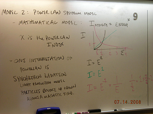
- Powerlaw spectrum model: in general, a mathematical model, but one interpretation is magnetic fields: charged particles move in circles or helix around magnetic fields, and this “bounce” up and down causes a different kind of spectrum to be emitted, that depends on the strength of the magnetic field and how the particles are moving.
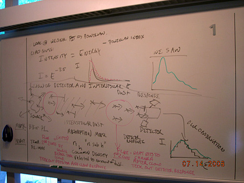
- Images of notes taken on these models: (blackbody notes, power law notes)
Fitting models to observations of visible light spectra for the sun and Crab nebula:
- Using Project LITE Spectrum Explorer, instructor demonstrates "fitting" a blackbody model and a power law model to the observation of the visible light spectrum of Sun, by adjusting parameter of each (Change temperature on blackbody, power law index on power law model.)
- Student challenge: Students "try to fit" both models to the blue region of the Crab nebula.
- Discuss: Which model gives a good fit? What do we mean by a good fit? (i.e. Model is not too far from the data.)
Fitting models to observations of X-ray spectra for neutron star RBS1223: Instructor(s), in small groups demonstrate fitting a blackbody model to isolated neutron star.
- Describe how BB model is appropriate: a neutron star is a hot object that light cannot pass through (opaque).
- Load X-ray light image (OBSID 731, Process: open specific obsid) and corresponding visible light image from "Analysis...Image Servers...SAO-DSS"
- Load previous "best looking" spectrum from ".dat" file created by histogram plot tool in Activity 2. Label axes properly. Y: Intensity (Photons detected in selected region), X: Energy (electron-volts)
- Choose approximately same region as in activity 2, and use CIAO/Sherpa spectral fit task to fit a blackbody model to the range 0.5 keV to 8 keV. (Process: fitting a model to data.)
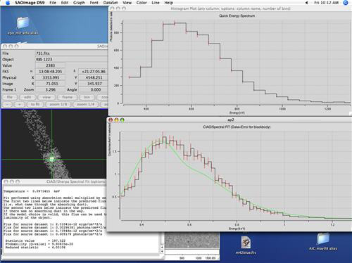
- Have students notice differences between original spectrum and spectrum fit output: higher energy bins are wider—computer chose them to have at least 20 counts/bin, Y axis is different units (counts/sec/keV), X-axis is different units (kilo-electron-volts).
- Save the output text to a file.
- Take an image of the whole screen, showing the X-ray, visible and two spectra. Save this image along with the text output into a word document. Write a short paragraph description of what the screenshot image is showing.
- See example screenshots for blackbody and power law fit here: (rbs1223 blackbody screenshot, rbs1223 power law screenshot)
- Student challenge: repeat exactly this entire process for blackbody fit. Then repeat the entire process while fitting a spectrum from the same region to a power law model.
- Students read and compare the fit outputs (images and text). They identify the most important differences between the two fits with their group, deciding as a group the 2 most important differences to share on the whiteboard. All groups then travel the room and "star" the differences they think are most important.
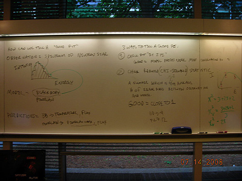
Wrap up discussion: What do we mean by a "good fit"
- Three parts to a "good fit": by eye (does model pass through all data point error bars?), "goodness of fit" parameter (a number close to 1, but not too much lower than 1), values of parameters (do they make physical sense?)
- In this case, blackbodyfit "looks closer", has better reduced chi-square statistic (= 5, instead of 12 with powerlaw), and realistic parameters (prediction is that amount of dust blocked only about 20% of flux, as opposed to a prediction that dust blocked 99.99% of flux, in other words, 1000 times more flux was actually emitted by the object, most of which was absorbed by dust.
- (Note: The amount of dust is measured by a quantity called "column density" which is the number of hydrogen atoms (typical "dust") which lie in a box between us and the objects, with the base of the box being a 1 cm x 1 cm square.)
- Image of notes about effects of dust and column density: (fitting models 1, fitting models 2)
Teacher tips/tricks:
- Timing: about 3-4 hours, but lots of time was spent on the video lectures.
- If students get overwhelmed at amount of material to repeat when fitting the blackbody model to the neutron star, break the steps into smaller chunks, having students help their group members if they get done early.
Assessment ideas:
- Analyze M81 (AGN) to see that the powerlaw spectrum would fit better. Summary of M81 fitting results: (M81 blackbody fit results (PDF), M81 powerlaw fit results (PDF)) Is there a reason why you would expect this? (AGN has strong magnetic fields near the supermassive black hole.)