
Extracting and Examining Spectra
Overview: Students create visible light and X-ray light spectra, first connecting the "rainbow" representation they are familiar with to the representation of a spectrum as a line on a graph of intensity versus energy.
Physical resources: Overhead projector, diffraction grating, blue (or other color) filter Electronic resources: Project LITE Spectrum Explorer
Representing spectra as histograms:
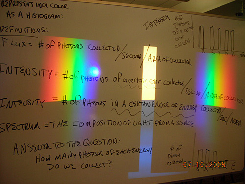
- Students review that light of 3 colors can combine to give white light, but then observe a rainbow coming from splitting white light with a diffraction grating from an overhead projector. Half of slit should be clear and other half can be covered with blue filter. Notes and example setup: (spectrum board)
- Brainstorm how we could represent this spectrum as a histogram...
- Recording the number of counts from each color, if we had a detector behind it would allow us to represent a spectrum as a histogram. This is a way to represent intensity of each color.
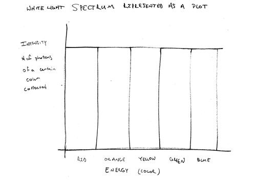
- We create a histogram above each spectrum, including the heights of the intensity, relative to one another.
- Instructor defines intensity, flux and spectrum.
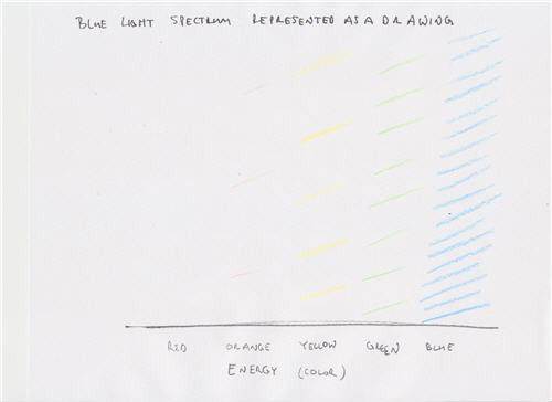
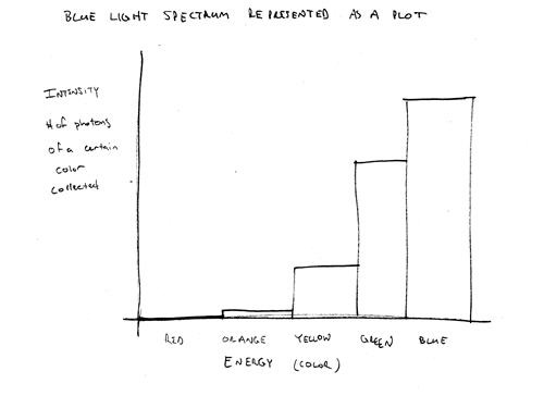
- Students represent the blue spectrum, using both colored pencil drawing and histogram plot.
- Instructor demonstrates the drawing tool in the (freeware) Project LITE "Spectrum Explorer" Java applet to draw the predicted histogram for the white light spectrum (i.e. a straight line), and compares the resulting "rainbow picture" with the actual projected spectrum. We see a spectrum with similar intensity across all colors.
- Students use the drawing tool in Project LITE to check that their prediction of the histogram actually reproduces the blue light spectrum.
- Students use Project LITE to examine recorded spectra from two different astronomical sources:
- Open sun spectrum ("Data file" button, then select "sun.dat" Set "X-axis range (eV) ... 0.1 to 6.2" to see the entire spectrum.) Ignore the dips for now.
- Open Crab Nebula blue region spectrum ("Astronomy" pull down menu to "Crab Nebula", then click on central "Crab Blue Region")
- Students should compare and contrast the two spectra in these representations. Have them record these differences and similarities using language from the particle model of light and using the new vocabulary "intensity," "energy," and "spectrum"
- Possible leading questions:
- What is different about the amount of blue (red, green, etc.) photons collected from the two objects?
- If an object looks blue in an image, does that mean we only collect blue photons from it?
- What would the spectrum look like if the sun had a smaller overall luminosity? (Histogram plot would be lower, and intensity would be less.)
- What's the difference between "sky blue" and "midnight blue" (difference in energy of photons collected) What's the difference between a high intensity blue and low intensity blue? (difference in number of photons collected) Why is it confusing to talk about "light blue" and "dark blue"? (What difference are you talking about? energy or intensity? It's often not clear...)
Extract X-ray spectra from Chandra images of 2 different X-ray light sources:
- Draw analogy between events file (listing of energy for each photon collected by Chandra) and restaurant file (listing of calories (energy) consumed by each person at the restaurant).
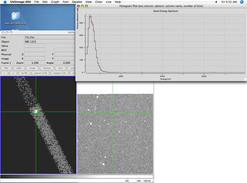
- Instructor demonstrates extracting spectrum for RBS1223 (obsid 731), an isolated neutron star.
- Load X-ray image, load corresponding visible light image: In ds9, click "Analysis...Image Servers...SAO-DSS" and click retrieve. This allows you access to the Digital Sky Survey.
- 'The "SAO-DSS Server" window allows you to retrieve an optical image of the field of your observation and load it into a new frame. The default retrieval image size and (RA,Dec) is equal to the size and center of the field currently displayed. You may also want to use the menus in the dialog box to select a different server for quicker access from your location.' (from "Using SAOimage ds9.")
- Use "Histogram plot" tool to specify energy range 300:8000:50, and check "use bin width instead of number of bins" (Process: Use histogram plot tool to extract a spectrum)
- Change plot to look like a histogram, using "step" linestyle: With "plot tool" window highlighted, click "View...Step" to add step linestyle, then click "View...Linear" to hide linear linestyle. ("Step" linestyle makes it easier to interpret the graph as a histogram.)
- Arrange the windows and take a screen shot of the analysis, shown here: (rbs1223 analysis screen shot)
- Save the x, y data file: With "plot tool" window highlighted, click "File...Save data" and name with ".dat" extension (so plot tool can recognize it when loading later)
- Load X-ray image, load corresponding visible light image: In ds9, click "Analysis...Image Servers...SAO-DSS" and click retrieve. This allows you access to the Digital Sky Survey.
- Challenge for students: repeat the demonstrated analysis
- In addition, extract spectra with different bin width: 50 eV, 100 eV, 200 eV and 400 eV
- Compare the difference between spectra, and explain why.
- Save the data they think looks best as .dat file.
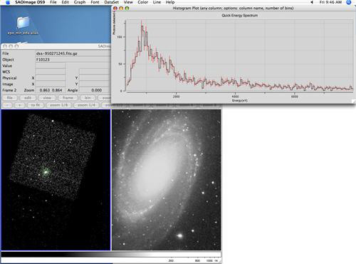
- Challenge: Students repeat entire process for M81 (obsid 5943), a galaxy with an active galactic nucleus (AGN), which is a supermassive black hole.
- Screen shot of analysis results: (m81 analysis screen shot)
- Extract spectra with different bin width: 50 eV, 100 eV, 200 eV and 400 eV
- Compare the difference between spectra, and explain why.
- Save the data they think looks best as .dat file.
- Students describe in notebooks or to another group what is different about the light collected from these 2 sources, in terms of both "color" and the particle model idea of counts.
- Possible comparison: Neutron star has high intensity (800 counts) in low energy photons (around 600 electron-volts), and AGN has a peak in intensity (around 100 counts) at a slightly higher energy (1000 electron-volts). We've collected photons of energy above 2000 electron-volts from the AGN, which the neutron star didn't even produce.
- Example of student comparison/contrast
Teacher tips/tricks:
- Timing: about 2 hours, but if needed, the analysis of M81 can be dropped. (The neutron star example is used again when describing how to fit spectrum observations to alternative models in activity 4.)
- Some mistakes from Summer 2008 to be sure not to repeat:
- Use the side of the spectrum which puts blue further to the right (higher energy), opposite to what is shown in this image. (spectrum board)
- When representing the spectra as a drawing with colored pencils, draw directly over the spectrum, making histogram bins all right next to each other, and then turn off the projector so students can see how the spectrum was represented. (This is important for the next note below.)
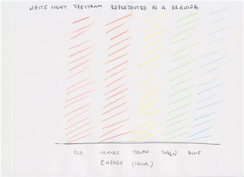
- When making the prediction of the blue spectrum, some students make the spectrum bands wider for more intense colors. When representing the complete spectrum for the first time in a drawing, be sure to make clear how to represent intensity. One suggestion is to color harder for higher intensity, or use colored slashes of different spacing, as shown in following images:
- Here are images of the drawing and plot representations of the white light spectrum and the blue light spectrum: (white light drawing, white light plot, blue light drawing, blue light plot)
- In addition, many students colored the histogram bins the same color, and even made the histogram bins different widths, which may indicate some confusion between the different representations.
- Working with Project LITE Spectrum Explorer: To make the spectrum representations ("rainbow images" and histogram plots) match with how we'll examine spectra from Chandra, use the following settings: "X-axis dimension...energy(eV)" and "X-axis range (eV)...1.78 to 3.1 (vis)" This will set up the energy range from low (red) to high (blue) energy.
Assessment ideas:
- Students are challenged to represent a different given spectrum as a drawing and/or histogram given by the instructor. They check themselves by using Project LITE Spectrum Explorer to draw the spectrum and then examine the resulting "rainbow" drawing representation.
- Show two different spectra, and have students interpret the differences between the light recieved from the sources, using the words "flux," "intensity," "energy," "counts" and the particle model of light, as well as the correct units.