2.2.5 Diffusion
Measurable Outcome 2.2, Measurable Outcome 2.5
In many engineering applications the dominant physical transport phenomenon is modeled as diffusion. A distinguishing feature of diffusion is that it results in mixing or mass transport, without requiring bulk motion. Thus, diffusion should not be confused with convection, which is a transport mechanism that utilize bulk motion to move particles from one place to another. In Latin, "diffundere" means "to spread out". In 1831, Thomas Graham studied diffusion in gases, and the main phenomenon was described by him:
"...gases of different nature, when brought into contact, do not arrange themselves according to their density, the heaviest undermost, and the lighter uppermost, but they spontaneously diffuse, mutually and equally, through each other, and so remain in the intimate state of mixture for any length of time."
Heat conduction is another example of diffusion, the diffusion of thermal energy. This section presents the conservation law for diffusion in differential form and discuss the behavior of problems modeled with diffusion. Diffusion is characterized by a flux,\(\vec{F}\) , of the form:
where \(\mu\) is the diffusion coefficient and \(U\) is the state. The differential form of the conservation law for the diffusion is,
Equation 2.33 is a second-order partial differential equation often called the diffusion equation or heat equation. Partial differential equations of this form arise in many applications including molecular diffusion and heat conduction.
One-dimensional Diffusion
We now illustrate the behavior of the diffusion equation considering a simple one-dimensional model problem. Consider the one-dimensional diffusion equation with constant \(\mu\). The diffusion equation simplifies to
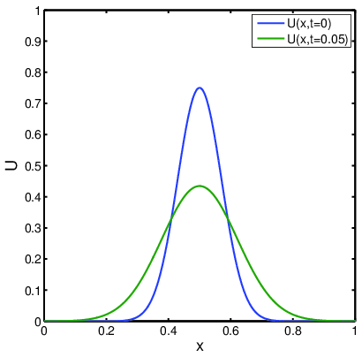
Figure 2.3 shows the initial condition
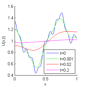
as well as the solution after a short time \(t=0.05\). The behavior of the diffusion equation is markedly different from what we have seen for the convection equation. The effect of the diffusion equation is to "smooth" out the conserved state in regions of steep gradients.
Unlike in the case of convection, (where the domain of dependence is along characteristics), the solution at any point \((\vec{x},t)\) for the diffusion equation depends on the solution everywhere else in the domain. Thus the domain of dependence at any point \((\vec{x}, t)\) is the entire domain at all previous time.