1.6.1 Nonlinear Systems
Measurable Outcome 1.1, Measurable Outcome 1.3, Measurable Outcome 1.6
For a system of ODE's, we have the same canonical form as for a scalar (see Equation 1.8),
except that \(u\) and \(f\) are vectors of the same length, \(d\):
Nonlinear Pendulum
One manner in which a system of ODE's occurs is for higher-order ODE's. A classic example of this is a second-order oscillator such as a pendulum. The nonlinear dynamics of a pendulum of length \(L\) satisfy the following second-order system of equations:
To transform this into a system of first-order equations, we define the angular rate, \(\omega\),
Then, Equation 1.86 becomes,
For this example,
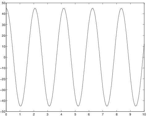
A forward Euler method was used to simulate the motion of a pendulum (with \(L\) = 1 m, \(g = 9.8\) m/sec\(^2\)) released from rest at an angle of \(45^\circ\) at a timestep of \({\Delta t}= 0.02\) seconds. The results are shown in Figure 1.8. While the oscillatory motion is evident, the amplitude is growing which is not expected physically. This would indicate some kind of numerical stability problem. Note, however, that if a smaller \({\Delta t}\) were used, the amplification would still be present but not as significant.
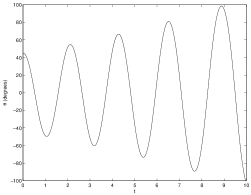
The same problem was also simulated using the midpoint method. These results are shown in Figure 1.9. For this method and \({\Delta t}\) choice, the oscillation amplitude is constant and indicates that the midpoint method is a better choice for this problem than the forward Euler method.