
2.2.3 Convection
Measurable Outcome 2.1, Measurable Outcome 2.2, Measurable Outcome 2.5
Convection is the concerted, collective movement of groups or aggregates of molecules within fluids. It is a transport mechanism of a substance or conserved property by a fluid due to the fluid's bulk motion. An example of convection is the transport of pollutants or silt in a river by bulk water flow downstream. Another commonly convected quantity is energy or enthalpy. Here the fluid may be any material that contains thermal energy, such as water or air. In general, any substance or conserved, extensive quantity can be convected by a fluid that can hold or contain the quantity or substance. Convection occurs on a large scale in atmospheres, oceans, planetary mantles, and it provides the mechanism of heat transfer for a large fraction of the outermost interiors of our sun and all stars. Fluid movement during convection may be invisibly slow, or it may be obvious and rapid, as in a hurricane. On astronomical scales, convection of gas and dust is thought to occur in the accretion disks of black holes, at speeds which may closely approach that of light.
In many applications, especially those in fluid dynamics, convection is the dominant physical transport mechanism over much of the domain of interest. While diffusion (see Section 2.2.5) is always present, often its effects are smaller except in limited regions (often near solid boundaries where boundary layers form due to the combined effects of diffusion and convection).
In this section, we will derive the convection equation using the conservation law as given in Equation 2.1. Specifically, let \(U\) be the 'conserved' scalar quantity, e.g., mass, energy, momentum, number of atoms or amount of "stuff" per unit volume, per unit area or per unit length. Let the flux of \(U\) be given by,
where \(\vec{v}(\vec{x},t)\) is a known velocity vector. This flux describes the amount of conserved quantity that, during a unit time, goes through a unit area (in 3 spatial dimensions), through a unit length (in 2 spatial dimensions), or through a point (in 1 spatial dimension). Note, we also use a zero source term, \(S=0\), a non-zero source term could be included, but for simplicity is assumed to be zero. As a PDE, this scalar conservation law is,
Expanding the spatial derivatives gives,
Often a reasonable assumption is that the velocity field is divergence free such that \(\nabla \cdot \vec{v} = 0\). In this case, we arrive at what is commonly referred to as the convection equation,
Physically, this equation states that following along the streamwise direction (i.e. convecting with the velocity), the quantity \(U\) does not change.
In developing numerical methods for convection-dominated problems, we will often rely on insight that can be gained from the convection equation for the specific case when the velocity field is a constant value, i.e. \(\vec{v}(\vec{x}, t) = \vec{v}\). In this situation, the solution to Equation 2.21 has the following form,
where \(U_0(\vec{x})\) is the distribution of \(U\) at time \(t=0\). By substitution, we can confirm that this indeed is a solution of Equation 2.21, Using the chain rule
, where \(\nabla _{\vec{x}}\) and \(\nabla _{\vec{\xi }}\) denote, respectively, the gradients with respect to \(\vec{x}\) and \(\vec{\xi }\). The partial derivatives of \(\vec{\xi }\) with respect to \(\vec{x}\) and \(r\) are,
where \(I\) is the identity tensor. Upon substitution of these partial derivatives,
Thus, \(U(\vec{x},t) = U_0(\vec{x}-\vec{v}t)\) is a solution to the convection equation.
Example One-dimensional Convection
To illustrate the behavior of the convection equation consider a simple one-dimensional convection problem
on the domain \(\Omega = [0,2]\), with constant flow velocity \(v=1\). The initial distribution \(U_0\) is
Figure 2.1 plots the initial solution \(U_0\) as well as \(U\) at \(t=1\).
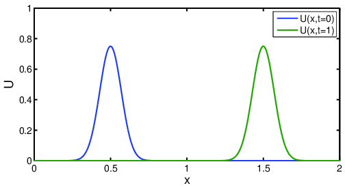
Looking at the solution for the one-dimensional convection problem, we observe that \(U(x,t)\) has the same shape as \(U_0(x)\), except the solution has been shifted by a distance \(v \times t\). This behavior in which the state \(U\) does not change as it propagates leads to the concept of a characteristic. A characteristic is defined as a trajectory \(\vec{x}(t)\) along which the state does not change. The rate-of-change of \(U\) along a trajectory \(\vec{x}(t)\) can be written using the total derivative as,
Comparing this to Equation 2.29, we see that if \(\frac{dx}{dt}=v\), then \(\frac{dU}{dt}=0\) (i.e., \(U=\) constant). In other words, the characteristic for the convection equation is a line with slope \(v\). Figure 2.2 shows the characteristic lines for the one-dimensional convection problem (in dashed lines) with the solutions at \(t=0\) and \(t=1\) superimposed. As we can see from Figure 2.2, the solution at \((x,t)\) is simply obtained by following the characteristic line back to \(t=0\) and evaluating the initial condition.
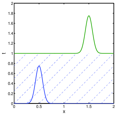
For convection and other equations which possess characteristics, the solution at a particular point in space and time \(U(\vec{x}, t)\) depends only upon the points along the characteristics from earlier times. For any partial differential equation, we call the region which affects the solution at \((\vec{x}, t)\)the domain of dependence. For convection, the domain of dependence for \((\vec{x},t)\) is simply the characteristic line, \(\vec{x}(t)\),\(s<t\).
Among other phenomena, this equation can model the convection of cars along a freeway. \(U\) is the number of cars per unit length of the freeway. There is with no entrance or exit ramps (source term) in the segment of freeway. The initial condition \(U(x, 0)\) is a distribution of cars at time \(t=0\). All cars are moving at velocity \(v\). So the flux, i.e., the number of cars that moves past a fixed spatial location per unit time, is \(v U\). At time \(t=1\) the distribution of cars, \(U(x,1)\), has shifted to the right, notice that the number of cars at point \(x\) at time \(t=1\) is the same as the number of cars at point \(x-vt\) at time \(t=0\). Notice that the car distribution \(at t=1\) does not depend on what is to the left or right of the characteristic.