2.9 Introduction to Finite Elements | Unit 2: Numerical Methods for Partial Differential Equations | Computational Methods in Aerospace Engineering | Aeronautics and Astronautics

2.9.1 Motivation

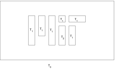
In this lecture, we introduce the finite element method (FEM). In its most general form, FEM is based on the method of weighted residuals. The application of the method of weighted residuals as described in Section 2.8.3 becomes difficult when the complexity of the problems increases, specifically in multiple dimensions and with varying properties (e.g., varying thermal conductivity in the heat diffusion problem). The heart of the difficulty in these applications is the construction of the weighted residual integrals. For the simple one-dimensional problem discussed in Section 2.8.3, these integrals were relatively easy to do. However, the analogous integrals in multiple dimensions with complex geometries are very difficult to evaluate without some additional form of numerical approximation. For example, consider the heat transfer problem shown in Figure 2.33 and imagine the difficulty in constructing a set of functions which satisfy the boundary conditions and then integrating the weighted residuals of these functions over the entire domain.

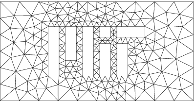
The figure spells out MIT using simple rectangles.

Figure 2.33: Heat transfer problem in a complex domain. Temperature at outer boundary is maintained at \(T_0\). Temperature of all of the internal rectangles except one are maintained at \(T_1\), while the remaining internal rectangle is maintained at \(T_2\).

The finite element method offers one approach to approximating the solution and the weighted residual integrals in general situations and, therefore, makes possible the approximation of complex physical problems. The basic idea behind the finite element method is to discretize the domain into small cells (called elements in FEM) and use these elements to approximate the solution and evaluate the weighted residuals (an example mesh can be seen in Figure 2.34). Typically, in each element, the solution is approximated using polynomial functions. Then, the weighted residuals are evaluated an element at a time and the resulting system of equations is solved to determine the weighting coefficients on the polynomials in each element.

This figure has the same rectangles spelling MIT as Figure 2.33, but the background is a complex mesh.

Figure 2.34: Mesh for heat transfer problem in a complex domain.

To introduce the basic concepts of the finite element method, we will first discuss the one-dimensional case. In future lectures, we will consider multiple dimensions and return to this complex heat transfer problem.