2.10 More on Finite Element Methods | Unit 2: Numerical Methods for Partial Differential Equations | Computational Methods in Aerospace Engineering | Aeronautics and Astronautics

2.10.1 Gaussian Quadrature

The finite element method requires the calculation of integrals over individual elements, for example,

\[\int _{x_{i}}^{x_{i+1}} {\phi _ i}_ x\, k \tilde{T}_ x\, dx, \quad \mbox{or} \quad \int _{x_{i}}^{x_{i+1}} {\phi _ i}\, f \, dx.\]

(2.221)

While in some settings these integrals can be calculated analytically, often they are too difficult. In this situation, numerical integration methods are used.

Gaussian quadrature is one of the most commonly applied numerical integration methods. Gaussian quadrature approximates an integral as the weighted sum of the values of its integrand. Consider integrating the general function \(g(\xi )\), over the domain \(-1 \leq \xi \leq 1\). Gaussian quadrature approximates this integral as a weighted sum of the values of \(g\) evaluated at discrete points over the domain:

\[\int _{-1}^{+1} g(\xi )\, d\xi \approx \sum _{q=1}^{N_ q} \alpha _ q g(\xi _ q). \label{equ:gq}\]

(2.222)

Here we have used \(N_ q\) quadrature points (i.e., integrand evaluations). \(\xi _ q\) is the location of the \(q\)th quadrature point in the domain and \(\alpha _ q\) is the corresponding quadrature weight.

Note that Gaussian quadrature rules are developed for specific integration limits, in this case between \(\xi = -1\) to \(+1\). Thus, for integration in an element, we will need to transform from \(x\) to \(\xi\).

Gaussian quadrature integration rules are determined by requiring exact integration of polynomial integrands, i.e., by considering integration of the function

\[g(\xi ) = c_0 + c_1\xi + c_2\xi ^2 + c_3\xi ^3 + \cdots + c_ M\xi ^ M,\]

(2.223)

for all values of the \(c_ m\) coefficients. Note that

\[\int _{-1}^{+1} \xi ^ m\, d\xi = \left\{ \begin{array}{cl} 0 & \mbox{if } m = \mbox{odd} \\[0.1in] \frac{2}{m+1} & \mbox{if } m = \mbox{even} \end{array}\right.\]

(2.224)

This gives us the result:

\[\int _{-1}^{+1} \sum _{m=0}^{M} c_ m\xi ^ m\, d\xi = 2\left(c_0 + \frac{1}{3}c_2 + \frac{1}{5}c_4 + \cdots \right). \label{equ:poly_ integral}\]

(2.225)

The \(N_ q = 1\) Quadrature Rule

For \(N_ q=1\), the quadrature rule is

\[\int _{-1}^{+1} g(\xi )\, d\xi \approx \alpha _1 g(\xi _1).\]

(2.226)

Now, using Equation (2.225), we determine the highest order polynomial that is integrable by a single quadrature point:

	\(\displaystyle 2\left(c_0 + \frac{1}{3}c_2 + \frac{1}{5}c_4 + \cdots \right)\)	\(\displaystyle =\)	\(\displaystyle \alpha _1 g(\xi _1)\)		(2.227)
		\(\displaystyle =\)	\(\displaystyle \alpha _1 \left(c_0 + c_1\xi _1 + c_2\xi _1^2 + c_3\xi _1^3 + \cdots + c_ M\xi _1^ M\right).\)		(2.228)

Matching term by term gives

	\(\displaystyle c_0\)	\(\displaystyle :\)	\(\displaystyle 2 = \alpha _1 \qquad \Rightarrow \alpha _1 = 2,\)		(2.229)
	\(\displaystyle c_1\)	\(\displaystyle :\)	\(\displaystyle 0 = \alpha _1\xi _1 \qquad \Rightarrow \xi _1 = 0.\)		(2.230)

Then, checking the \(c_2\) term shows that it is not integrated exactly. So, with one point, a linear polynomial is the highest order polynomial that can be evaluated exactly and the quadrature rule is

\[\int _{-1}^{+1} g(\xi )\, d\xi \approx \alpha _1 g(\xi _1), \qquad \alpha _1 = 2, \quad \xi _1 = 0.\]

(2.231)

The \(N_ q = 2\) Quadrature Rule

For \(N_ q=2\), the quadrature rule is,

\[\int _{-1}^{+1} g(\xi )\, d\xi \approx \alpha _1 g(\xi _1) + \alpha _2 g(\xi _2).\]

(2.232)

Again using Equation (2.225), we determine the highest order polynomial that is integrable by two quadrature points:

\(\displaystyle 2\left(c_0 + \frac{1}{3}c_2 + \frac{1}{5}c_4 + \cdots \right)\)	\(\displaystyle =\)	\(\displaystyle \alpha _1 g(\xi _1) + \alpha _2 g(\xi _2)\)	(2.233)
	\(\displaystyle =\)	\(\displaystyle \alpha _1 \left(c_0 + c_1\xi _1 + c_2\xi _1^2 + c_3\xi _1^3 + \cdots + c_ M\xi _1^ M\right) +\)	(2.234)
		\(\displaystyle \alpha _2 \left(c_0 + c_1\xi _2 + c_2\xi _2^2 + c_3\xi _2^3 + \cdots + c_ M\xi _2^ M\right).\)	(2.235)

Matching the first four terms gives the following constraints:

\(\displaystyle c_0\)	\(\displaystyle :\)	\(\displaystyle 2 = \alpha _1 + \alpha _2,\)	(2.236)
\(\displaystyle c_1\)	\(\displaystyle :\)	\(\displaystyle 0 = \alpha _1\xi _1 + \alpha _2\xi _2,\)	(2.237)
\(\displaystyle c_2\)	\(\displaystyle :\)	\(\displaystyle \frac{2}{3} = \alpha _1\xi _1^2 + \alpha _2\xi _2^2,\)	(2.238)
\(\displaystyle c_3\)	\(\displaystyle :\)	\(\displaystyle 0 = \alpha _1\xi _1^3 + \alpha _2\xi _2^3.\)	(2.239)

These constraints can be met by choosing

\[\alpha _1 = \alpha _2 = 1, \quad \xi _1 = -\frac{1}{\sqrt {3}}, \quad \xi _2 = \frac{1}{\sqrt {3}}.\]

(2.240)

Thus, this rule will integrate cubic polynomials exactly.

Calculation of Forcing Integral with Gauss Quadrature

We wish to apply Gaussian quadrature to evaluate the forcing integral,

\[\int _{x_{i}}^{x_{i+1}} {\phi _ i}\, f \, dx. \label{equ:wf}\]

(2.241)

Remember that this is the last term in the definition of the weighted residual for our diffusion problem, Equation (2.211).

To do this, we first transform between the \(x\) and \(\xi\) space. For this integral in element \(i\), the transformation is

\[x(\xi ) = x_{i} + \frac{1}{2}(1+\xi )(x_{i+1}-x_ i), \quad \Rightarrow dx = \frac{1}{2}(x_{i+1}-x_ i)d\xi .\]

(2.242)

Substitution in the forcing integral gives

\[\int _{x_{i}}^{x_{i+1}} \phi _ i \, f \, dx = \int _{-1}^{+1} \frac{1}{2}(x_{i+1}-x_ i) \phi _ i \, f \, d\xi , \qquad \Rightarrow \qquad g(\xi ) = \frac{1}{2}(x_{i+1}-x_ i)\, \phi _ i[x(\xi )]\, f[x(\xi )].\]

(2.243)

Note that the dependence of \(\phi _ i\) and \(f\) on \(\xi\) is shown through the dependence of these functions on \(x = x(\xi )\). However, for the basis functions, it is often easier to directly determine \(\phi _ i\) from \(\xi\). For example, in the case of linear polynomial basis functions, the basis functions with element \(i\) can be written as

	\(\displaystyle \phi _1(\xi )\)	\(\displaystyle =\)	\(\displaystyle \frac{1}{2}(1-\xi ),\)		(2.244)
	\(\displaystyle \phi _2(\xi )\)	\(\displaystyle =\)	\(\displaystyle \frac{1}{2}(1+\xi ).\)		(2.245)

Clearly, these functions vary linearly with \(\xi\). \(\phi _1(\xi )\) is one at \(\xi =-1\) and decreases linearly to zero at \(\xi =+1\). \(\phi _2(\xi )\) is zero at \(\xi =-1\) and increases linearly to one at \(\xi =+1\).

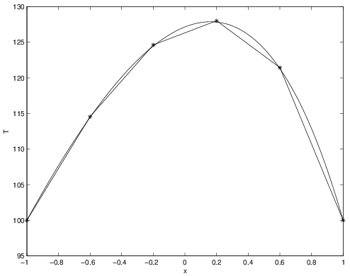
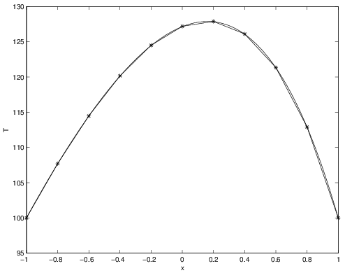
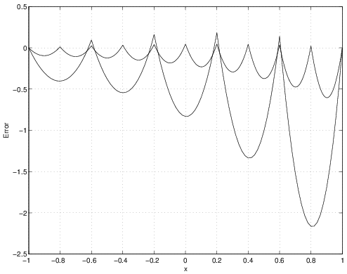
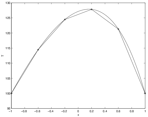
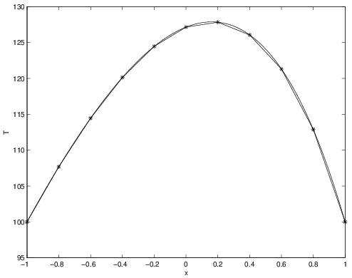
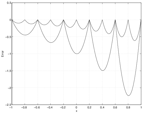
The following is a MATLAB^® script that uses Gaussian quadrature to evaluate the forcing integral and solve the problem described in Section 2.8.1. The number of points being used is set at the beginning of the script. Results for both 1-point and 2-point quadrature are shown in Figures 2.41-2.46 for \(5\) and \(10\) elements. While the 2-point quadrature rule has lower error than the 1-point rule, both appear to be second-order accurate since the errors reduce by nearly a factor of \(4\) for the factor 2 change in mesh size. Also, the results are no longer exact at the nodes like they were in Section 2.9.3 (though the 2-point quadrature rules are quite close).

% FEM solver for d2T/dx2 + f = 0 where f = 50 exp(x)
%
% BC's: T(-1) = 100 and T(1) = 100.
%
% Gaussian quadrature is used in evaluating the forcing integral.
%
% Note: the finite element degrees of freedom are
%       stored in the vector T.

% Number of elements
nElem = 5;
x = linspace(-1,1,nElem+1);

% Set quadrature rule
Nq = 2;
if (Nq == 1),
  alphaq(1) = 2.0; xiq(1) = 0.0;
elseif (Nq == 2),
  alphaq(1) = 1.0; xiq(1) = -1/sqrt(3);
  alphaq(2) = 1.0; xiq(2) =  1/sqrt(3);
else
  fprintf('Error: Unknown quadrature rule (Nq = %i)\n',Nq);

  return;
end

% Zero stiffness matrix
K = zeros(nElem+1, nElem+1);
F = zeros(nElem+1, 1);

% Loop over all elements and calculate stiffness and residuals
for elem = 1:nElem,

  n1 = elem;
  n2 = elem+1;

  x1 = x(n1);
  x2 = x(n2);

  dx = x2 - x1;

  % Add contribution to n1 weighted residual due to n1 function
  K(n1, n1) = K(n1, n1) - (1/dx);

  % Add contribution to n1 weighted residual due to n2 function
  K(n1, n2) = K(n1, n2) + (1/dx);

  % Add contribution to n2 weighted residual due to n1 function
  K(n2, n1) = K(n2, n1) + (1/dx);

  % Add contribution to n2 weighted residual due to n2 function
  K(n2, n2) = K(n2, n2) - (1/dx);

  % Evaluate forcing term using quadrature
  for nn = 1:Nq,

    % Get xi location of quadrature point
    xi = xiq(nn);

    % Calculate x location of quadrature point
    xq = x1 + 0.5*(1+xi)*dx;

    % Calculate f
    f = 50*exp(xq);

    % Calculate phi1 and phi2
    phi1 = 0.5*(1-xi);
    phi2 = 0.5*(1+xi);

    % Add forcing term to n1 weighted residual
    F(n1) = F(n1) - alphaq(nn)*0.5*phi1*f*dx;

    % Add forcing term to n2 weighted residual
    F(n2) = F(n2) - alphaq(nn)*0.5*phi2*f*dx;

  end

end

% Set Dirichlet conditions at x=-1
n1 = 1;
K(n1,:)    = zeros(size(1,nElem+1));
K(n1, n1)  = 1.0;
F(n1)      = 100.0;

% Set Dirichlet conditions at x=1
n1 = nElem+1;
K(n1,:)    = zeros(size(1,nElem+1));
K(n1, n1)  = 1.0;
F(n1)      = 100.0;

% Solve for solution
T = K\F;


% Plot solution
figure(1);
plot(x,T,'*-');
xlabel('x');
ylabel('T');

% For the exact solution, we need to use finer spacing to plot
% it correctly.  If we only plot it at the nodes of the FEM mesh,
% the exact solution would also look linear between the nodes.  To
% make sure there is always enough resolution relative to the FEM
% nodes, the size of the vector for plotting the exact solution is
% set to be 20 times the number of FEM nodes.
Npt = 20*nElem+1;
xe = linspace(-1,1,Npt);
Te = -50*exp(xe) + 50*xe*sinh(1) + 100 + 50*cosh(1);
hold on; plot(xe,Te); hold off;

% Plot the error.  To do this, calculate the error on the same
% set of points in which the exact solution was plot.  This
% requires that the location of the point xx(i) be found in the
% FEM mesh to construct the true solution at this point by linearly
% interpolating between the two nodes of the FEM mesh.

Terr(1) = T(1) - Te(1);
h = x(2)-x(1);
for i = 2:Npt-1,
  xxi = xe(i);
  Tei = Te(i);
  j = floor((xxi-xe(1))/h) + 1;
  x0 = x(j);
  x1 = x(j+1);
  T0 = T(j);
  T1 = T(j+1);
  xi = 2*(xxi - x0)/(x1-x0)-1;  % This gives xi between +/-1
  Ti = 0.5*(1-xi)*T0 + 0.5*(1+xi)*T1;
  Terr(i) = Ti - Tei;
end
Terr(Npt) = T(nElem+1) - Te(Npt);

figure(2);
plot(xe,Terr);
xlabel('x');
ylabel('Error');

This graph shows two very similar lines, each with a single peak, that represent the exact solution and the finite element solution using Nq=1 point Gaussian quadrature with 5 elements.

Figure 2.41: Comparison of finite element solution using \(N_ q=1\) point Gaussian quadrature with \(N=5\) elements to the exact solution.

Figure 2.42: Comparison of finite element solution using \(N_ q=1\) point Gaussian quadrature with \(N=10\) elements to the exact solution.

This graph shows two lines of inverted peaks representing the error between the exact and finite element solution with Gaussian quadrature using Nq=1 points. There are twice as many and smaller inverted peaks for the 5 element line than the 10 element line.

Figure 2.43: Error between exact solution and finite element solutions (\(N=5\) and \(N=10\)) with Gaussian quadrature using \(N_ q=1\) points.

This graph shows two very similar lines, each with a single peak, that represent the exact solution and the finite element solution using Nq=2 point Gaussian quadrature with 5 elements.

Figure 2.44: Comparison of finite element solution using \(N_ q=2\) point Gaussian quadrature with \(N=5\) elements to the exact solution.

Figure 2.45: Comparison of finite element solution using \(N_ q=2\) point Gaussian quadrature with \(N=10\) elements to the exact solution.

Figure 2.46: Error between exact solution and finite element solutions (\(N=5\) and \(N=10\)) with Gaussian quadrature using \(N_ q=2\) points.