
2.6.1 Upwinding
Measurable Outcome 2.2, Measurable Outcome 2.5, Measurable Outcome 2.6, Measurable Outcome 2.9
Consider the one-dimensional convection equation,
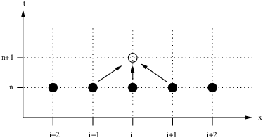
For simplicity, we will consider the specific case in which \(u>0\). Recall that for the convection equation, the solution \(U(x,t)\) is obtained by following the characteristic line back to the inditial condition and evaluating \(U_0(\xi )\) where \(\xi = x-ut\). For the case of \(u>0\) this means that the solution at \((\hat{x}, \hat{t})\) only depend on the locations to the left of \(\hat{x}\) and for tmes before \(\hat{t}\). Since the convection equation has some inherent directionality, it is natural for our numerical scheme to also have some sort of directional bias. First consider the FTCS method. The solution \(U_ i^{n+1}\) is updated as:
This is graphically depicted in Figure 2.16. This numerical scheme has no inherent directionality as it uses a derivative approximation that is centered, taking equal (magnitude) weights from nodes to the left and right.
Now consider the Forward Time-Backward Space (FTBS) method. It uses the backwards difference formula \(\delta _ x^{-}U_ i\), and gives the update
The method is graphically depicted in Figure 2.17.
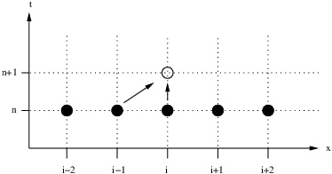
Notice that the numerical scheme is now biased to upstream values. The upstream direction is the left in this case, because the characteristic lines travel towards the right as time increases. (The upstream direction would be the right if the characteristic lines travel towrads the left as time increases.) Numerical schemes which exhibit such an upstream bias are called upwind schemes. Thus, the FTBS method is also known as the first-order upwind scheme. Not that when \(u<0\) then the forward difference \(\delta _ x^{+}U_ i = (U_{i+1}-U_{i})/\Delta x\) leads to the correct upwind scheme.
Exercise
Which of the following is a second-order accurate upwind difference of \(U_{x_ i}\) (assume positive convection velocity)?