2.2.6 Convection-Diffusion
Measurable Outcome 2.1, Measurable Outcome 2.2, Measurable Outcome 2.5
In practice, both convection and diffusion are important phenomenon governing fluid dynamics. While convection may be the dominant transport mechanism in most of a flow, accounting for diffusion near solid boundaries may be essential for accurately computing engineering quantities such as drag or heat transfer. The convection-diffusion equation is derived from a general conservation law including both convective and diffusive fluxes. In differential form, the convection-diffusion equation is
The convection-diffusion equation arises in many engineering applications ranging from heat transfer to statistical mechanics (and even in finance!). Solutions of the convection-diffusion equation exhibit behavior which is the combined effect of both convection and diffusion. A key question which naturally arises is how significant are the relative effects of convection and diffusion. This is governed by the non-dimensional Peclet number (in aerodynamics applications, the Reynolds number is equivalent).
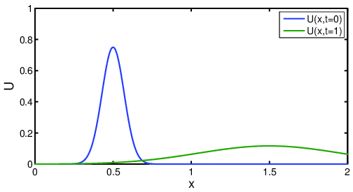
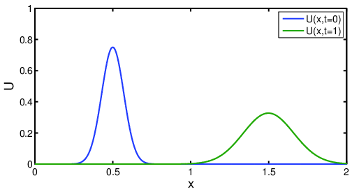
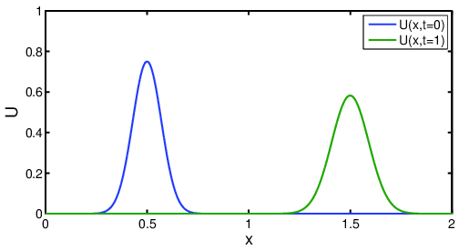
where \(L\) is a characteristic length scale for the problem of interest. When \(Pe \ll 1\) diffusion effects are dominant, and convection plays a relatively small role. On the other hand, when \(Pe \gg 1\) convection is the dominant transport mechanism. Figures 2.5, 2.6, 2.7 show solutions for the one-dimensional convection-diffusion problem with Peclet numbers \(10, 100\) and \(1000\) (\(\vec{v}=1\) is fixed). As the Peclet number increases the solution of the convection-diffusion problem approaches that of the pure convection problem.