2.9.3 1-D Linear Elements and the Nodal Basis
The finite element method typically uses polynomial functions inside each element. Furthermore, the approximation is usually required to be continuous from element to element. The simplest element which permits continuous functions would be to assume linear variations of \(x\) inside each element. This type of element is called a linear element (not too surprisingly). Using linear finite elements, a sample solution might look like that shown in Figure 2.36.
A linear function can be described by two degrees of freedom. For example, a linear function within an element could be uniquely determined by the following combinations of information:
-
the function values at the two endpoints (i.e., nodes) of the element,
-
the function value at some point in the element and the function slope in the element.
For a mesh composed of \(N\) elements, a total of \(N+1\) degrees of freedom exist to describe a continuous, piecewise linear function. If the approximation were allowed to be discontinuous from element to element, then there would be \(2N\) degrees of freedom but continuity removes \(N-1\) degrees of freedom (one per internal node). Thus, the degrees of freedom to describe a solution over a domain discretized into \(N\) linear elements could be (among other choices),
-
the values of the function at the \(N+1\) nodes,
-
the value of the function at some point in the domain and the slopes in the \(N\) elements.
The first choice is the most common and leads to what is known as the nodal basis.
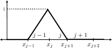
We now derive the nodal basis functions (i.e., the \(\phi _ j(x)\)) for linear elements. As discussed above, for \(N\) linear elements we have \(N+1\) degrees of freedom and therefore \(N+1\) basis functions, i.e.,
where \(a_ j\) are the \(N+1\) degrees of freedom. For a nodal basis, we choose \(a_ j = \tilde{T}(x_ j)\). Substituting this into Equation (2.199) gives,
Now, evaluating this expansion at node \(i\),
Finally, since the solutions vary linearly over each element, this means that \(\phi _ j(x)\) is zero for \(x < x_{j-1}\) and \(x > x_{j+1}\), increases linearly from zero to one from \(x_{j-1}\) to \(x_{j}\), and decreases linearly back to zero at \(x_{j+1}\). \(\phi _ j(x)\) is shown in Figure 2.37. The, specific function is,