2.9 Introduction to Finite Elements

2.9.6 Calculation of the Stiffness Matrix

Measurable Outcome 2.12, Measurable Outcome 2.14, Measurable Outcome 2.15, Measurable Outcome 2.16, Measurable Outcome 2.17, Measurable Outcome 2.20

For the steady diffusion problem we have been considering in this chapter, the finite element method results in a linear system of equations of the form

\[Ka = F,\]

(2.220)

where \(K\) is commonly referred to as the stiffness matrix. The unknown coefficients \(a_ i\) of the solution approximation are in the vector \(a\). The right-hand side vector \(F\) represents the term \(\int _{-L/2}^{L/2} \phi _ j f dx\) as well as boundary conditions. The calculation of \(K\) and \(F\) for the finite element method is commonly performed by looping over each element and sending the contributions from each element to the proper entry in \(K\) and \(F\).

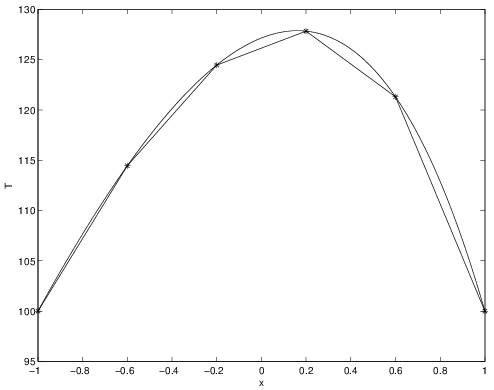
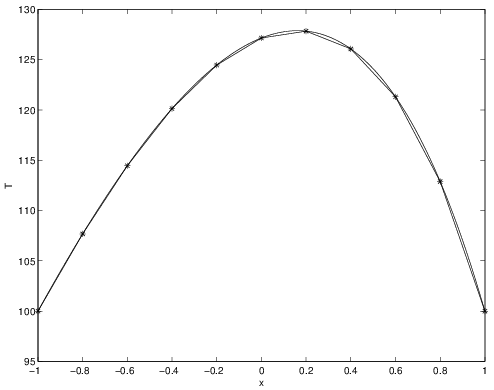
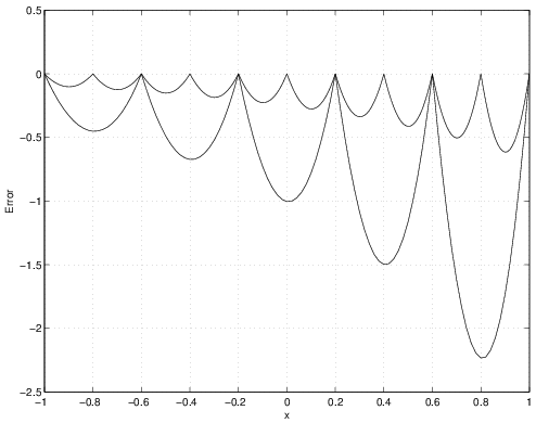
The MATLAB^® implementation of the finite element method for the problem described in Section 2.8.1 is shown below. Note, at the bottom of the script the exact solution and the error in the finite element solution are calculated and plotted. Interestingly, the FEM results for linear elements are exact at the nodes. This in general is not true, and is only a result of this specific problem. However, in between the nodes (i.e., within the elements), there is error since a linear function is being used to represent a higher-order (curved) solution. The error, \(\tilde{T}(x)-T(x)\), is shown in Figure 2.40 for both \(N=5\) and \(N=10\) solutions. Note: to construct this plot, each element was subdivided into 20 points and the FEM and exact solution were calculated at these points and compared.

% FEM solver for d2T/dx2 + f = 0 where f = 50 exp(x)
%
% BCs: T(-1) = 100 and T(1) = 100.
%
% Note: the finite element degrees of freedom are
%       stored in the vector T.

% Number of elements
nElem = 10;
x = linspace(-1,1,nElem+1);

% Zero stiffness matrix
K = zeros(nElem+1, nElem+1);
F = zeros(nElem+1, 1);

% Loop over all elements and calculate stiffness and residuals
for elem = 1:nElem,

  n1 = elem;
  n2 = elem+1;

  x1 = x(n1);
  x2 = x(n2);

  dx = x2 - x1;

  % Add contribution to n1 weighted residual due to n1 function
  K(n1, n1) = K(n1, n1) - (1/dx);

  % Add contribution to n1 weighted residual due to n2 function
  K(n1, n2) = K(n1, n2) + (1/dx);

  % Add contribution to n2 weighted residual due to n1 function
  K(n2, n1) = K(n2, n1) + (1/dx);

  % Add contribution to n2 weighted residual due to n2 function
  K(n2, n2) = K(n2, n2) - (1/dx);

  % Add forcing term to n1 weighted residual
  F(n1) = F(n1) - (50*(exp(x2)-x2*exp(x1) + x1*exp(x1) - exp(x1))/dx);

  % Add forcing term to n2 weighted residual
  F(n2) = F(n2) - (50*(x2*exp(x2)-exp(x2)-x1*exp(x2)+exp(x1))/dx);

end


% Set Dirichlet conditions at x=-1
n1 = 1;
K(n1,:)    = zeros(size(1,nElem+1));
K(n1, n1) = 1.0;
F(n1)      = 100.0;


% Set Dirichlet conditions at x=1
n1 = nElem+1;
K(n1,:)    = zeros(size(1,nElem+1));
K(n1, n1) = 1.0;
F(n1)      = 100.0;


% Solve for solution
T = K\F;


% Plot solution
figure(1);
plot(x,T,'*-');
xlabel('x');
ylabel('T');

% For the exact solution, we need to use finer spacing to plot
% it correctly.  If we only plot it at the nodes of the FEM mesh,
% the exact solution would also look linear between the nodes.  To
% make sure there is always enough resolution relative to the FEM
% nodes, the size of the vector for plotting the exact solution is
% set to be 20 times the number of FEM nodes.
Npt = 20*nElem+1;
xe = linspace(-1,1,Npt);
Te = -50*exp(xe) + 50*xe*sinh(1) + 100 + 50*cosh(1);
hold on; plot(xe,Te); hold off;

% Plot the error.  To do this, calculate the error on the same
% set of points in which the exact solution was plot.  This
% requires that the location of the point xx(i) be found in the
% FEM mesh to construct the true solution at this point by linearly
% interpolating between the two nodes of the FEM mesh.

Terr(1) = T(1) - Te(1);
h = x(2)-x(1);
for i = 2:Npt-1,
  xxi = xe(i);
  Tei = Te(i);
  j = floor((xxi-xe(1))/h) + 1;
  x0 = x(j);
  x1 = x(j+1);
  T0 = T(j);
  T1 = T(j+1);
  xi = 2*(xxi - x0)/(x1-x0)-1;  % This gives xi between +/-1
  Ti = 0.5*(1-xi)*T0 + 0.5*(1+xi)*T1;
  Terr(i) = Ti - Tei;
end
Terr(Npt) = T(nElem+1) - Te(Npt);

figure(2);
plot(xe,Terr);
xlabel('x');
ylabel('Error');

Exercise