2.8 Method of Weighted Residuals

2.8.3 The Method of Weighted Residuals

Measurable Outcome 2.12, Measurable Outcome 2.13, Measurable Outcome 2.14

While the collocation method enforces the residual to be zero at \(N\) points, the method of weighted residuals requires \(N\) weighted integrals of the residual to be zero. A weighted residual is simply the integral over the domain of the residual multiplied by a weight function, \(w(x)\). For example, in the one-dimensional diffusion problem we are considering, a weighted residual is,

\[\int _{-1}^{1} w(x)\, R(\tilde{T},x)\, dx.\] (2.174)

By choosing \(N\) weight functions, \(w_ i(x)\) for \(i=1,\ldots ,N\), and setting these \(N\) weighted residuals to zero, we obtain \(N\) equations which we solve to determine the \(N\) unknown values of \(a_ j\).

We define the weighted residual for \(w_ i(x)\) to be

\[R_ i(\tilde{T}) \equiv \int _{-1}^{1} w_ i(x)\, R(\tilde{T},x)\, dx.\] (2.175)

The method of weighted residuals requires

\[R_ i(\tilde{T}) = 0 \qquad \mbox{for } i=1,\ldots ,N.\] (2.176)

In the method of weighted residuals, the next step is to determine appropriate weight functions. A common approach, known as the Galerkin method, is to set the weight functions equal to the functions used to approximate the solution. That is,

\[w_ i(x) = \phi _ i(x). \quad \mbox{(Galerkin)}.\] (2.177)

For the heat diffusion example we have been considering, this would give weight functions as

  \(\displaystyle w_1(x)\) \(\displaystyle =\) \(\displaystyle (1-x)(1+x),\)   (2.178)
  \(\displaystyle w_2(x)\) \(\displaystyle =\) \(\displaystyle x(1-x)(1+x).\)   (2.179)

Now, we must calculate the weighted residuals. For our example, we have

  \(\displaystyle R_1(\tilde{T})\) \(\displaystyle =\) \(\displaystyle \int _{-1}^{1} w_1(x)\, R(\tilde{T},x)\, dx,\)   (2.180)
    \(\displaystyle =\) \(\displaystyle \int _{-1}^{1} (1-x)(1+x)\, \left(-2 a_1 - 6 a_2 x + 50 e^ x\right)\, dx,\)   (2.181)
    \(\displaystyle =\) \(\displaystyle -\frac{8}{3} a_1 + 200 e^{-1}.\)   (2.182)

To do this integral, the following results were used:

  \(\displaystyle \int _ a^ b (1-x)(1+x)\, dx\) \(\displaystyle =\) \(\displaystyle \left[ x - \frac{1}{3}x^3 \right]_ a^ b,\)   (2.183)
  \(\displaystyle \int _ a^ b x(1-x)(1+x)\, dx\) \(\displaystyle =\) \(\displaystyle \left[ \frac{1}{2}x^2 - \frac{1}{4}x^4 \right]_ a^ b,\)   (2.184)
  \(\displaystyle \int _ a^ b x^2 e^ x\, dx\) \(\displaystyle =\) \(\displaystyle \left[ x^2 e^ x - 2 x e^ x + 2 e^ x \right]_ a^ b.\)   (2.185)

Similarly, calculating \(R_2\):

  \(\displaystyle R_2(\tilde{T})\) \(\displaystyle =\) \(\displaystyle \int _{-1}^{1} w_2(x)\, R(\tilde{T},x)\, dx,\)   (2.186)
    \(\displaystyle =\) \(\displaystyle \int _{-1}^{1} x(1-x)(1+x)\, \left(-2 a_1 - 6 a_2 x + 50 e^ x\right)\, dx,\)   (2.187)
    \(\displaystyle =\) \(\displaystyle -\frac{8}{5} a_2 + 100 e^{1} - 700 e^{-1},\)   (2.188)

where the following results have been used:

  \(\displaystyle \int _ a^ b x^2(1-x)(1+x)\, dx\) \(\displaystyle =\) \(\displaystyle \left[ \frac{1}{3}x^3 - \frac{1}{5}x^5 \right]_ a^ b,\)   (2.189)
  \(\displaystyle \int _ a^ b x e^ x\, dx\) \(\displaystyle =\) \(\displaystyle \left[ x e^ x - e^ x \right]_ a^ b,\)   (2.190)
  \(\displaystyle \int _ a^ b x^3 e^ x\, dx\) \(\displaystyle =\) \(\displaystyle \left[ x^3 e^ x - 3 x^2 e^ x + 6x e^ x - 6e^ x \right]_ a^ b.\)   (2.191)

Finally, we can solve for \(a_1\) and \(a_2\) by setting the weighted residuals \(R_1\) and \(R_2\) to zero:

  \(\displaystyle -\frac{8}{3} a_1 + 200 e^{-1}\) \(\displaystyle =\) \(\displaystyle 0,\)   (2.192)
  \(\displaystyle -\frac{8}{5} a_2 + 100 e^{1} - 700 e^{-1}\) \(\displaystyle =\) \(\displaystyle 0.\)   (2.193)

This could be written as a \(2\times 2\) matrix equation and solved, but the equations are decoupled and can be readily solved,

\[\Rightarrow \left(\begin{array}{c} a_1 \\ a_2 \end{array}\right) = \left(\begin{array}{r} 75 e^{-1} \\ \frac{125}{2}e^{1} - \frac{875}{2}e^{-1} \end{array}\right) = \left(\begin{array}{r} 27.591 \\ 8.945 \end{array}\right).\] (2.194)

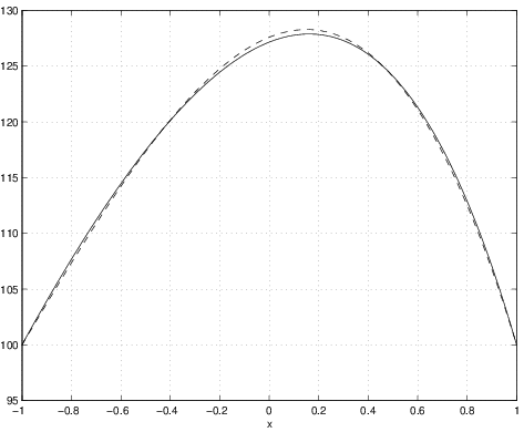
The results using this method of weighted residuals are shown in the figures below. Comparison with the collocation method results shows that the method of weighted residuals is more accurate in this case.

This graph shows two very similar lines, each with a single peak, that represent the results T and ~T for method of weighted residuals.
Figure 2.30: Comparison of \(T\) (solid) and \(\tilde{T}\) (dashed) for method of weighted residuals.
This graph has one line, representing the error T minus ~T for method of weighted residuals.  The line begins at the y-axis point zero, then decreases below -0.3, increases above 0.4, then decreases to almost -0.4, and finally increases back to zero.
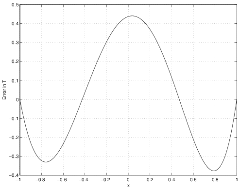
Figure 2.31: Error \(\tilde{T}-T\) for method of weighted residuals.
This graph of the residual R(~T, x) for method of weighted resiuduals has a single line that steadily decreases and then increases.
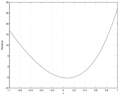
Figure 2.32: Residual \(R(\tilde{T},x)\) for method of weighted residuals.