1.2.5 The Midpoint Method
Measurable Outcome 1.5, Measurable Outcome 1.6
Now, let's look at another integration method known as the midpoint method. For this method, we will use a slightly different point of view to derive it. Specifically, let's start from the definition of a derivative,
Now, instead of taking the limit, assume a finite \({\Delta t}\). Then, we end up with an approximation to \(du/dt\):
Then, we can re-arrange this to the following estimate for \(u(t+{\Delta t})\),
Then, following the same process as in the forward Euler method, we arrive at the midpoint method,
However, because of the use of \(v^{n-1}\), the midpont method can only be applied for \(n \geq 1\). Thus, for the first timestep a different numerical method must be applied (e.g. the forward Euler method).
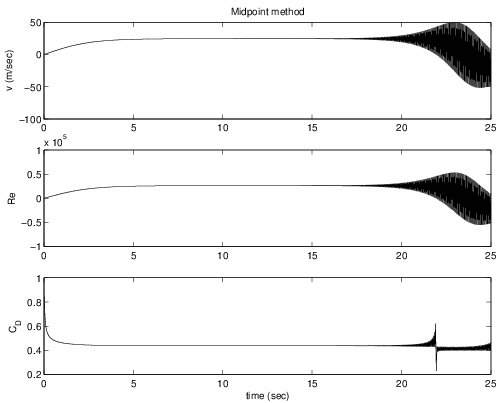
We will now solve the falling ice problem using the midpoint method. Using the same values of \({\Delta t}\) and \(T\) as before, the results are shown in Figure 1.3.
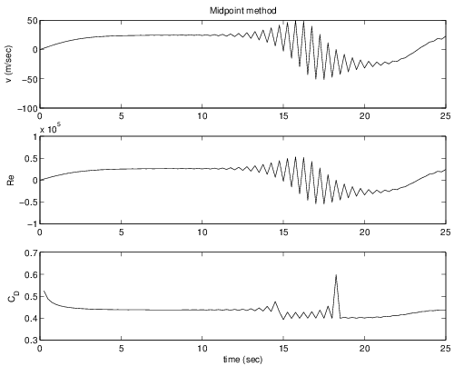
Clearly, something has gone wrong here as the results show non-physical oscillations. Perhaps the oscillations will disappear if we take a smaller timestep. To test out this hypothesis, let's re-run the midpoint method with \({\Delta t}= 0.025\, sec\) which is one-tenth the previous timestep. Those results are shown in Figure 1.4. Unfortunately, while the results are better, the oscillations are clearly still present. For this problem, clearly the forward Euler method is a better choice than the midpoint method. We will see why this has happened in a few lectures.