
1.2.3 Discretization
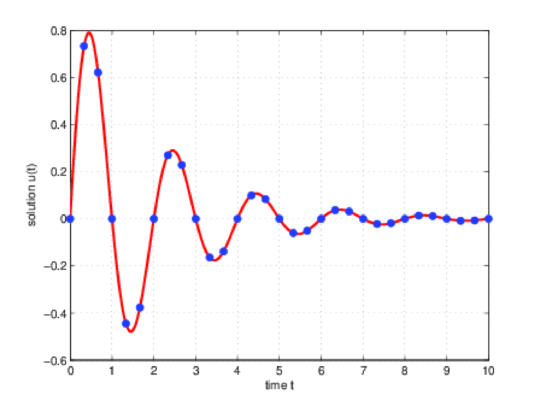
When you plot the solution in MATLAB®, you are likely creating two vectors: one corresponding to points in time \(t=[t_0, t_1, \ldots ,t_ N]\) and another corresponding to the solution \(\mathbf{u}(t)= [u(t_0),u(t_1),\ldots ,u(t_ N)]\) at those points in time. This process of representing a continuous function by a finite set of numbers is referred to as discretization. The main idea is illustrated in Figure 1.1. Instead of representing the function continuously, we represent it as a finite set of ordered pairs \((t_ n, u(t_ n))\).
When we solve mathematical problems on a computer, it will always be necessary to discretize them. For initial value problems, we will begin with the initial condition \(u_0\) at time \(t=0\) and solve forward in time. First we select a time step \({\Delta t}>0\) representing the length of the interval between any two adjacent time points \(t_ n\) and \(t_{n+1}\). Although it is not necessary to choose a constant \({\Delta t}\) for the entire simulation, this is the approach we will take for this course. (You should be aware that state of the art numerical simulation codes adaptively select the time step, e.g., based on an estimate of the error.) Our numerical solution will then involve computing an approximation to the solution \(u(t_ n)\) using information up to (and sometimes including, see implicit methods) time step \(n\).