1.2.4 The Forward Euler Method
Measurable Outcome 1.5, Measurable Outcome 1.6
We now consider our first numerical method for ODE integration, the forward Euler method. The general problem we wish to solve is to approximate the solution \(u(t)\) for Equation 1.8 with an appropriate initial condition, \(u(0) = u_0\). Usually, we are interested in approximating this solution over some range of \(t\), say from \(t = 0\) to \(t = T\). Or, we may not know a precise final time but wish to integrate forward in time until an event occurs (e.g. the problem reaches a steady state). In either case, the basic philosophy of numerical integration using finite difference methods is to start from a known initial state, \(u(0)\), and somehow approximate the solution a small time forward, \(u({\Delta t})\) where \({\Delta t}\) is a small time increment. Then, we repeat this process and move forward to the next time to find, \(u(2{\Delta t})\), and so on. Initially, we will consider the situation in which \({\Delta t}\) is fixed for the entire integration from \(t=0\) to \(T\). However, the best methods for solving ODE's tend to be adaptive methods in which \({\Delta t}\) is adjusted depending on the current approximation.
Before moving on to the specific form of the forward Euler method, let's put some notations in place. Superscripts will be used to indicate a particular iteration, that is \(t^ n\) denotes the time at iteration \(n\). Thus, assuming constant \({\Delta t}\),
The approximation from the numerical integration will be defined as \(v\). Thus, using the superscript notation,
Now, let's derive the forward Euler method. There are several ways to motivate the forward Euler method. We will start with an approach based on Taylor series. Specifically, the Taylor expansion of \(u(t^{n+1})\) about \(t^ n\) is,
Using only the first two terms in this expansion,
Finally, the term \(u_ t(t^ n)\) is in fact just \(f(u(t^ n),t^ n)\) since the governing equation is Equation 1.8. Thus,
Since we do not know \(u(t^ n)\), we will instead use the approximation from the previous timestep, \(v^ n\). Thus, the forward Euler algorithm is,
and \(v^0 = u(0)\).
Falling Ice Problem
Now, let's apply the forward Euler method to solving the falling sphere problem. Suppose the sphere is actually a small particle of ice falling in the atmosphere at an altitude of approximately 3000 meters. Specifically, let's assume the radius of the particle is \(a = 0.01 m\). Then, since the density of ice is approximately \(\rho _ p = 917 \, kg/m^3\), the mass of the particle can be calculated from,
At that altitude, the properties of the atmosphere are:
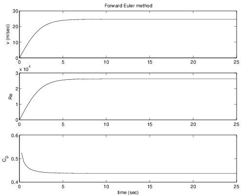
We expect the particle to accelerate until it reaches its terminal velocity which will occur when the drag force is equal to the gravitational force. But, a priori, we do not know how long that will take (in class, we will discuss some ways to make this estimate). For now, let's set \(T= 25\, sec\) and use a timestep of \({\Delta t}= 0.25\, sec\). The results are shown in Figure 1.2.