
3.3.3 Monte Carlo Example
Measurable Outcome 3.3, Measurable Outcome 3.5
To demonstrate the Monte Carlo simulation method in more detail, let's consider the specific case where the thermal barrier coating in the previous turbine blade example is known to be uniformly distributed from \(0.00025m < L_{TBC} < 0.00075m\) as shown from the probability density function (PDF) of LTBC in Figure 3.3.
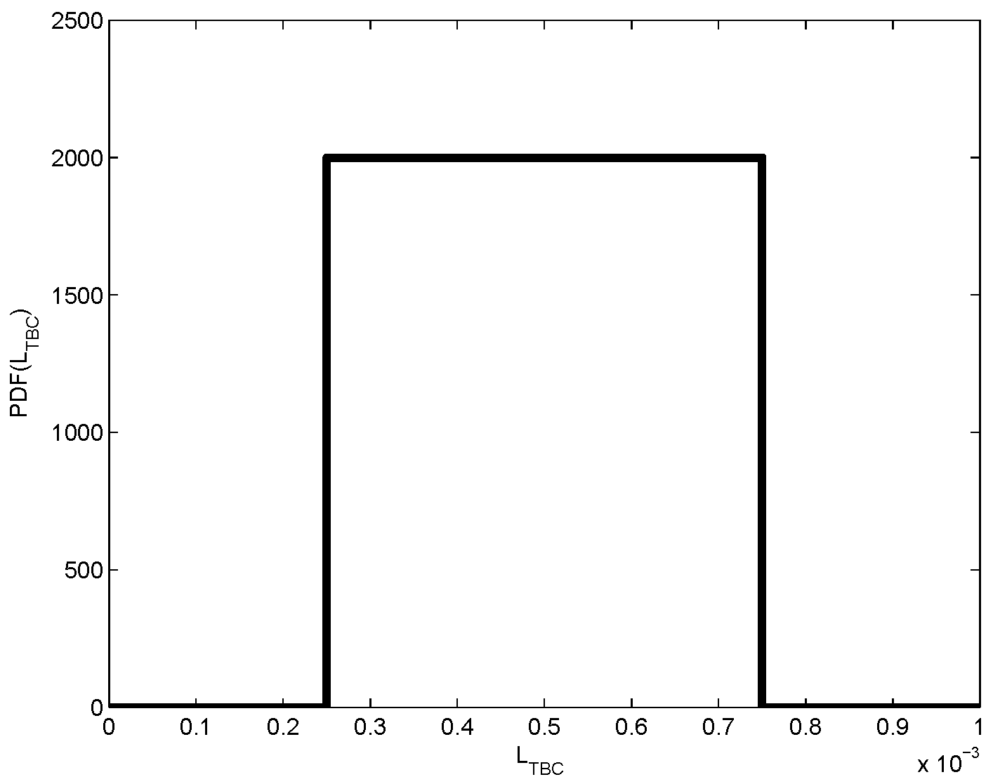
The first step is to generate a random sample of \(L_{TBC}\). The basic approach relies on the ability to generate random numbers that are uniformly distributed from 0 to 1. This type of functionality exists within many different scientific programming environments or languages. In MATLAB®, the command rand returns a random number that is uniformly distributed from 0 to 1. Then, using the uniform distribution from 0 to 1, a uniform distribution of \(L_{TBC}\) over the desired range can be created,
where \(U\) is a random variable uniformly distributed from 0 to 1.
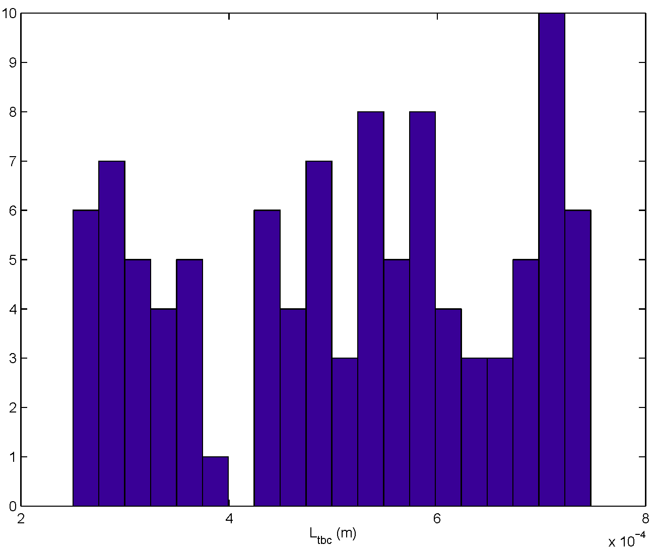
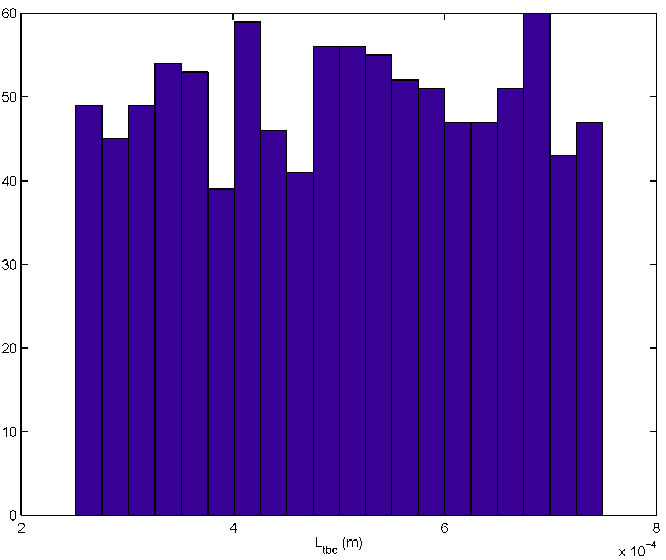
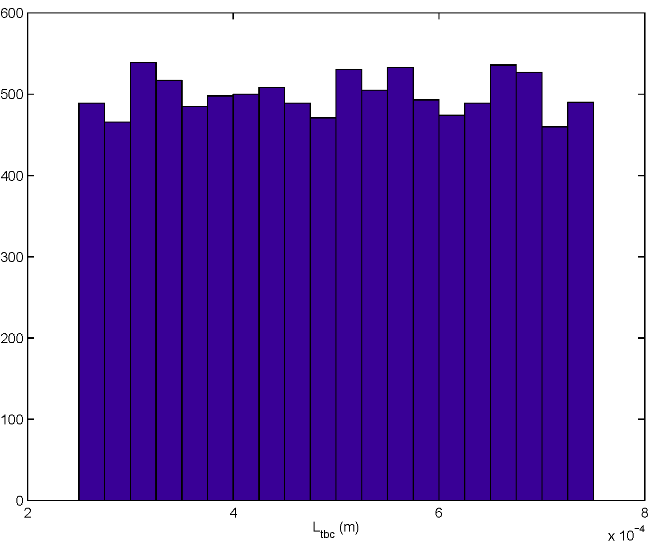
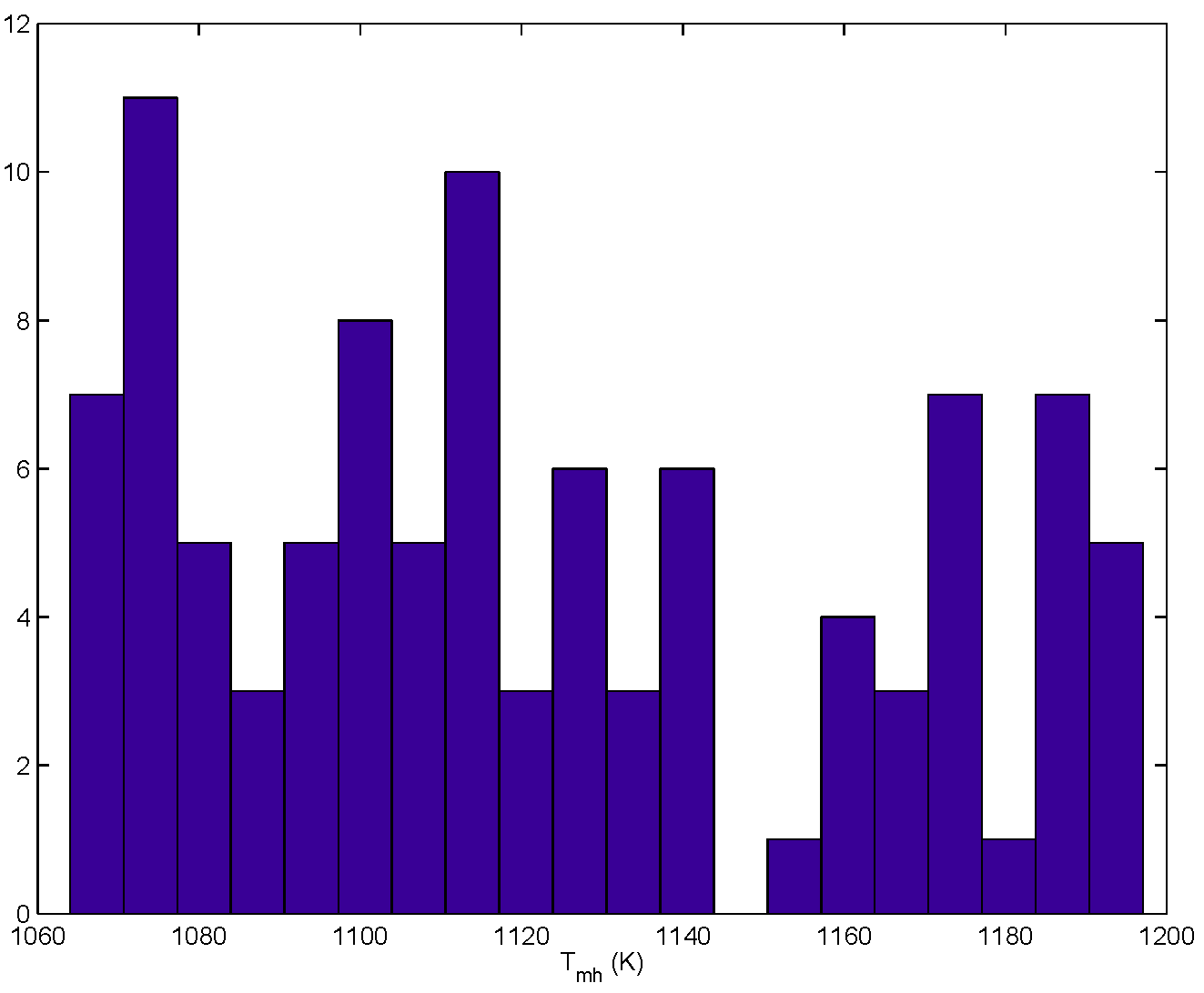
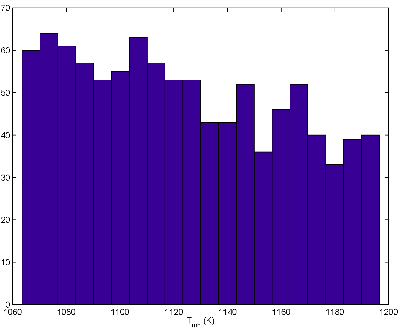
This approach is used to create the samples shown as histograms in Figure 21.3 for samples of size \(N\) = 100, 1000, and 10000. For the smaller sample size (specifically \(N\) = 100), the fact that the sample was drawn from a uniform distribution is not readily apparent. However, as the number of samples increases, the uniform distribution becomes more evident. Clearly, the sample size will have a direct impact on the accuracy of the probabilistic estimates in the Monte Carlo method.
The following is a MATLAB script that implements the Monte Carlo method for this uniform distribution of \(L_{TBC}\). The distributions of \(T_{mh}\) shown in Figure 3.5 correspond to the \(L_{TBC}\) distributions shown in Figure 3.4 and were generated with this script.
clear all;
hgas = 3000;
Tgas = 1500;
ktbc = 1;
km = 20;
Lm = 0.003;
hcool = 1000;
Tcool = 600;
N = 100;
Ltbc = zeros(N,1);
Tmh = zeros(N,1);
for n = 1:N, Ltbc(n) = 0.00025 + 0.0005*rand;
[Ttbc, Tmh(n), Tmc, q] = blade1D(hgas, Tgas, ktbc, Ltbc(n), km, Lm, hcool, Tcool);
end figure(1);
hist(Ltbc,20);
xlabel('\(L_{tbc}\) (m)');
figure(2);
hist(Tmh,20);
xlabel('\(T_{mh}\) (K)');
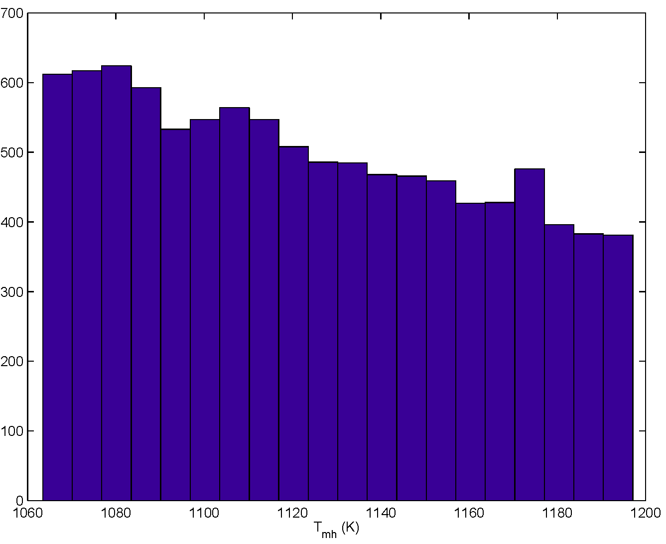
Consider the third plot in Figure 3.5. If we choose a sample corresponding to \(L_{TBC}\)=3, in which region of the output histogram do you expect the corresponding \(T_{mh}\) to lie ?
For any given value of \(L_{TBC}\), \(T_{mh}\) is inversely proportional to \(L_{TBC}\), the thicker the barrier coating, the lower \(T_{mh}\) will be.