
3.3.4 Inversion Method for Sampling
Input variability can be distributed in many ways beyond the simple uniform distribution considered above. In this section, we discuss a common approach used to implement the Monte Carlo method for non-uniform distributions. However, we note that for many of the most common distribution types, random number generators are widely available. For example, in MATLAB, the function randn returns random numbers that are normally distributed with a mean of zero and a standard deviation of one. In MATLAB's Statistics Toolbox, many other distribution types are available (see the documentation for the random function for details).
Inversion Method for Generating Random Numbers
In these notes, we will discuss the inversion method for generating random numbers with non-uniform distributions. While other methods exist for generating random numbers, they are often based on the inversion method. The basic principle of the inversion method is to utilize the inverse of the cumulative distribution function (CDF) to transform a uniform distribution to a desired distribution. Recall that the CDF is defined as the integral of the PDF,
and that the CDF is related to probability by,
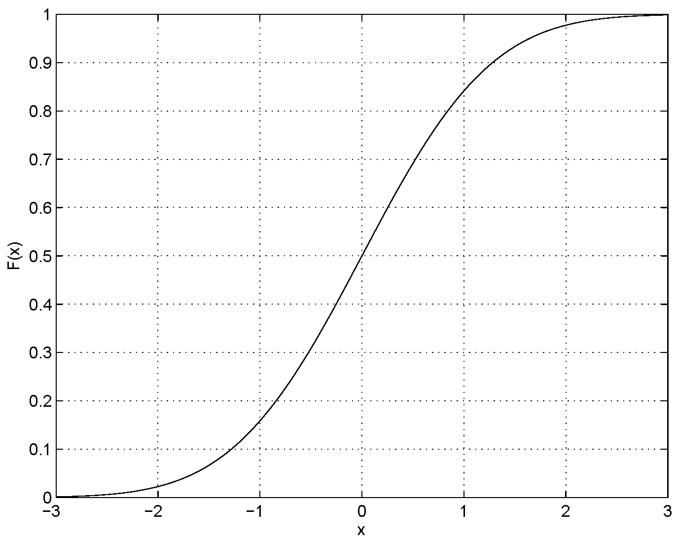
That is, the probability of the random variable \(X \leq x\) is the CDF evaluated at \(x\). As shown in Figure 3.6, \(F(x)\) ranges from 0 to 1.
The inversion method for generating random numbers of an arbitrary distribution consists of the following two steps:
-
Generate a random number, \(u\), from a uniform distribution between 0 and 1.
-
Given \(u\), find the value of \(x\) at which \(u=F(x)\). In other words, invert \(F(x)\) such that, \(x=F^{-1}(u)\).
Sampling Triangular Distributions
A triangular distribution is defined by the parameters \(x_{min}\), the minimum value of \(x\), \(x_{mpp}\), the most-probable value of \(x\), and \(x_{max}\), the maximum value of \(x\). The cumulative distribution function (CDF) of a triangular distribution is,
for \(x_{min} < x < x_{mpp}\), and
for \(x_{mpp} < x < x_{max}\). Given a percentile drawn from a uniform random distribution, \(u=F(x_ u)\), the value \(x_ u\) can be found by inverting the previous relationships for \(F(x)\). Specifically, note that,
Thus, if \(u < F(x_{mpp})\) then \(x_{min} < x < x_{mpp}\), we invert Equation 21.1 to find,
Otherwise, if \(u > F(x_{mpp})\) then \(x_{mpp} < x < x_{max}\), we invert Equation 21.2 to find,
Consider a triangular distribution with the following parameters, \(x_{min}\) = 0, \(x_{max}\) = 1 and \(x_{mpp} = \frac{1}{2}\), which we want to draw a sample from. Suppose we sample a \(U[0,1]\) and obtain \(u=\frac{3}{4}\), the corresponding sample from the triangular distribution \(x_ u\) is,
\(F(\frac{1}{2})\) = \(\frac{1}{2}\), the drawn \(u > F(\frac{1}{2})\) and hence we can use Equation 21.2, which gives \(x_ u= 1 - \frac{1}{\sqrt {8}}\).