
1.8.3 Backwards Differentiation Methods
Measurable Outcome 1.12, Measurable Outcome 1.15, Measurable Outcome 1.17, Measurable Outcome 1.18, Measurable Outcome 1.19
Backwards differentiation methods are some of the best multi-step methods for stiff problems. The backwards differentiation formulae are of the form,
The coefficients for the first through fourth order methods are given in the table below.
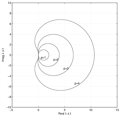
The stability boundary for these methods are shown below. As can be seen, all of these methods are stable everywhere on the negative real axis, and are mostly stable in the left-half plane in general. Thus, backwards differentiation work well for stiff problems in which stong damping is present.
MATLAB®'s ODE Integrators
MATLAB has a a set of tools for integration of ODE's. We will briefly look at two of them: ode45 and ode15s. ode45 is designed to solve problems that are not stiff while ode15s is intended for stiff problems. ode45 is based on a four and five-stage Runge-Kutta integration (discussed in Section 1.9), while ode15s is based on a range of highly stable implicit integration formulas (one option when using ode15s is to use the backwards differentiation formulas). As a short illustration on how these MATLAB ODE integrators are implemented, the following script solves the one-dimensional diffusion problem from Section 1.7.1 using either ode45 or ode15s. The specific problem we consider here is a bar which is initially at a temperature \(T_{init} = 400 K\) and at \(t=0\), the temperature at the left and right ends is suddenly raised to \(800 K\) and \(1000 K\), respectively.
% MATLAB script: dif1d_main.m
%
% This code solve the one-dimensional heat diffusion equation
% for the problem of a bar which is initially at T=Tinit and
% suddenly the temperatures at the left and right change to
% Tleft and Tright.
%
% Upon discretization in space by a finite difference method,
% the result is a system of ODE's of the form,
%
% u_t = Au + b
%
% The code calculates A and b.  Then, uses one of MATLAB's
% ODE integrators, either ode45 (which is based on a Runge-Kutta
% method and is not designed for stiff problems) or ode15s (which
% is based on an implicit method and is designed for stiff problems).
%

clear all; close all;

sflag = input('Use stiff integrator? (1=yes, [default=no]): ');

% Set non-dimensional thermal coefficient
k   = 1.0; % this is really k/(rho*cp)

% Set length of bar
L = 1.0; % non-dimensional

% Set initial temperature
Tinit = 400;

% Set left and right temperatures for t>0
Tleft = 800;
Tright = 1000;

% Set up grid size
Nx = input(['Enter number of divisions in x-direction: [default=' ...
            '51]']);
if (isempty(Nx)),
  Nx = 51;
end

h  = L/Nx;
x  = linspace(0,L,Nx+1);

% Calculate number of iterations (Nmax) needed to iterate to t=Tmax
Tmax = 0.5;

% Initialize a sparse matrix to hold stiffness & identity matrix
A = spalloc(Nx-1,Nx-1,3*(Nx-1));
I = speye(Nx-1);

% Calculate stiffness matrix

for ii = 1:Nx-1,

  if (ii > 1),
    A(ii,ii-1) = k/h^2;
  end

  if (ii < Nx-1),
    A(ii,ii+1) = k/h^2;
  end

  A(ii,ii) = -2*k/h^2;

end

% Set forcing vector
b = zeros(Nx-1,1);
b(1)    = k*Tleft/h^2;
b(Nx-1) = k*Tright/h^2;

% Set initial vector
v0 = Tinit*ones(1,Nx-1);

if (sflag == 1),

  % Call ODE15s
  options = odeset('Jacobian',A);
  [t,v] = ode15s(@dif1d_fun,[0 Tmax],v0,options,A,b);

else

  % Call ODE45
  [t,v] = ode45(@dif1d_fun,[0 Tmax],v0,[],A,b);

end

% Get midpoint value of T and plot vs. time
Tmid = v(:,floor(Nx/2));
plot(t,Tmid);
xlabel('t');
ylabel('T at midpoint');
As can be seen, this script pre-computes the linear system \(A\) and the column vector \(b\) since the forcing function for the one-dimensional diffusion problem can be written as the linear function, \(f = Av + b\). Then, when calling either ODE integrator, the function which returns \(f\) is the first argument in the call and is named, dif1d_fun. This function is given below:
% MATLAB function: dif1d_fun.m
%
% This routine returns the forcing term for
% a one-dimensional heat diffusion problem
% that has been discretized by finite differences.
% Note that the matrix A and the vector b are pre-computed
% in the main driver routine, dif1d_main.m, and passed
% to this function.  Then, this function simply returns
% f(v) = A*v + b.  So, in reality, this function is
% not specific to 1-d diffusion.

function [f] = dif1d_fun(t, v, A, b)

f = A*v + b;
As can be seen from dif1d_fun, \(A\) and \(b\) have been passed into the function and thus the calculation of \(f\) simply requires the multiplication of \(v\) by \(A\) and the addition of \(b\).
The major difference between the implementation of the ODE integrators in MATLAB and our discussions is that MATLAB's implementations are adaptive. Specifically, MATLAB's integrators estimate the error at each iteration and then adjust the timestep to either improve the accuracy (i.e. by decreasing the timestep) or efficiency (i.e. by increasing the timestep).
The results for the stiff integrator, ode15s are shown in Figure 1.22.
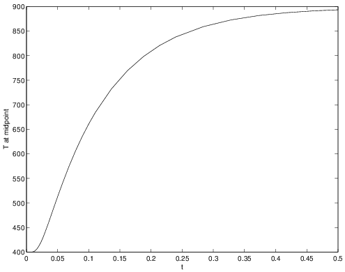
These results look as expected (note: in integrating from \(t=0\) to \(t=0.5\), a total of 64 timesteps were taken).
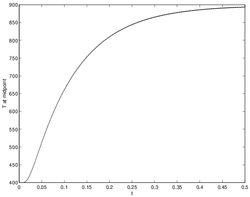
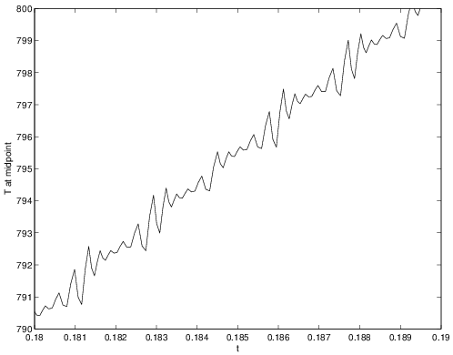
The results for the non-stiff integrator are shown in Figure 1.23 and in a zoomed view in Figure 1.24. The presence of small scale oscillations can be clearly observed in the ode45 results. These oscillations are a result of the large negative eigenvalues which require small \({\Delta t}\) to maintain stability. Since the ode45 method is adaptive, the timestep automatically decreases to maintain stability, but the oscillatory results clearly show that the stability is barely achieved. Also, as a measure of the relative inefficiency of the ode45 integrator for this stiff problem, note that 6273 timesteps were required to integrate from \(t=0\) to \(t=0.5\).
One final concern regarding the efficiency of the stiff integrator ode15s. In order for this method to work in an efficient manner for large systems of equations such as in this example, it is very important that the Jacobian matrix, \({\partial f}/{\partial u}\) be provided to MATLAB. If this is not done, then ode15s will construct an approximation to this derivative matrix using finite differences and for large systems, this will become a significant cost. In the script dif1d_main, the Jacobian is communicated to the ode15s integrator using the odeset routine. Note: ode45 is an explicit method and does not need the Jacobian so it is not provided in that case.