
1.8.2 Adams-Moulton Methods
Measurable Outcome 1.12, Measurable Outcome 1.15, Measurable Outcome 1.17, Measurable Outcome 1.18, Measurable Outcome 1.19
Adams-Moulton methods are implicit methods of the form,
These methods use the same time derivative approximation as the Adams-Bashforth methods, however they include the \(n+1\) value of \(f\).
Table 3: Coefficients for Adams-Moulton methods. Note: the \(p=1\) method is the backward Euler method, and the \(p=2\) method is the Trapezoidal method.
The coefficients for the first through fourth order methods are given in the table above.
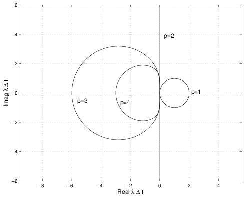
Figure 1.20: Adams-Moulton stability regions for \(p=1\) through \(p=4\) methods. Note: \(p=1\) is stable outside of contour, the \(p=2\) integrator is stable in the left-half plane, and \(p\geq 3\) are stable inside their respective contours.
The stability boundary for these methods are shown in Figure 1.20. While the stability regions are larger than the Adams-Bashforth methods, for \(p>2\) the methods have bounded stability regions. Thus, they will not be appropriate for stiff problems.