2.11 The Finite Element Method for Two-Dimensional Diffusion

2.11.2 Reference Element and Linear Elements

Measurable Outcome 2.15, Measurable Outcome 2.16

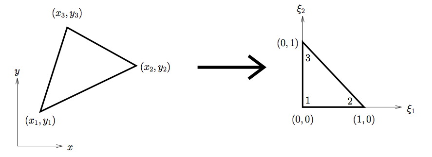
In multiple dimensions, a common practice in defining the polynomial functions within an element is to transform each element into a canonical, or so-called “reference" element. Figure 2.47 shows the mapping commonly used for triangular elements which maps a generic triangle in \((x,y)\) into a right triangle in \((\xi _1, \xi _2)\).

A tilted triangle representing a polynomial function in space is shown on the left.  This triangle is rotated in multiple dimensions (x and y) to transform the triangle into a right triangle representing the reference element on the right.
Figure 2.47: Transformation of a generic triangular element in \((x,y)\) into the reference element in \((\xi _1,\xi _2)\).

In the reference element space, the nodal basis for linear polynomials will be one at one of the nodes, and reduce linearly to zero at the other nodes. These functions are

  \(\displaystyle \phi _1(\xi _1, \xi _2)\) \(\displaystyle =\) \(\displaystyle 1 - \xi _1 - \xi _2, \label{equ:phi1_2d}\)   (2.262)
  \(\displaystyle \phi _2(\xi _1, \xi _2)\) \(\displaystyle =\) \(\displaystyle \xi _1, \label{equ:phi2_2d}\)   (2.263)
  \(\displaystyle \phi _3(\xi _1, \xi _2)\) \(\displaystyle =\) \(\displaystyle \xi _2. \label{equ:phi3_2d}\)   (2.264)

Then, within the element, the solution \(\tilde{T}\) in the \((\xi _1,\xi _2)\) space is the combination of these three basis functions multiplied by the corresponding nodal coefficients,

\[\tilde{T}(\xi _1,\xi _2) = \sum _{j=1}^{3} a_ j \phi _ j(\xi _1,\xi _2). \label{equ:Txi}\] (2.265)

Using Equation (2.265), the value of \(\tilde{T}\) can be found at any \((\xi _1,\xi _2)\). To find the \((x,y)\) locations in terms of the \((\xi _1, \xi _2)\), we can expand them using the nodal locations and the nodal basis functions, i.e.,

\[\vec{x}(\xi _1,\xi _2) = \sum _{j=1}^{3} \vec{x}_ j \phi _ j(\xi _1,\xi _2).\] (2.266)

Since the \(\phi _ i(\xi _1,\xi _2)\) are linear functions of \(\xi _1\) and \(\xi _2\), this amounts to a linear transformation between \((\xi _1,\xi _2)\) and \((x,y)\). Specifically, substituting the nodal basis functions gives

  \(\displaystyle \vec{x}(\xi _1,\xi _2)\) \(\displaystyle =\) \(\displaystyle \vec{x}_1 \left(1 - \xi _1 - \xi _2\right) + \vec{x}_2\xi _1 + \vec{x}_3\xi _2,\)   (2.267)
  \(\displaystyle \Rightarrow \vec{x}(\xi _1,\xi _2)\) \(\displaystyle =\) \(\displaystyle \vec{x}_1 + \left(\vec{x}_2-\vec{x}_1\right)\xi _1 + \left(\vec{x}_3-\vec{x}_1\right)\xi _2.\)   (2.268)

This can be written in a matrix notation as,

\[\left(\begin{array}{c} x \\ y \end{array}\right) = \left(\begin{array}{c} x_1 \\ y_1 \end{array}\right) + \left(\begin{array}{cc} x_2-x_1 & x_3-x_1 \\ y_2-y_1 & y_3-y_1\end{array}\right) \left(\begin{array}{c} \xi _1 \\ \xi _2 \end{array}\right) \label{equ:xi_ to_ x}\] (2.269)

This equation can be inverted to also determine \((\xi _1,\xi _2)\) as a function of \((x,y)\),

\[\left(\begin{array}{c} \xi _1 \\ \xi _2 \end{array}\right) = \left(\begin{array}{cc} x_2-x_1 & x_3-x_1 \\ y_2-y_1 & y_3-y_1\end{array}\right)^{-1} \left(\begin{array}{c} x-x_1 \\ y-y_1 \end{array}\right) \label{equ:x_ to_ xi}\] (2.270)