2.8.2 The Collocation Method
Measurable Outcome 2.12, Measurable Outcome 2.13
One approach to determine the \(N\) unknown values of \(a_ j\) would be to enforce the governing PDE at \(N\) spatial points in the domain (i.e., to make sure that the the approximate solution exactly satisfies the PDE at \(N\) points). Note that in general, the exact solution will not be a linear combination of the \(\phi _ j(x)\), so it will not be possible for our approximate solution to satisfy the PDE at every point in the domain. To see this, let's substitute our approximate solution \(\tilde{T}(x)= 100 + a_1 \phi _1(x) + a_2 \phi _2(x)\) into Equation 2.149. First, let's derive an expression for \(\tilde{T}_{xx}\):
Next, we define a residual for Equation 2.149,
The residual tells us by how much the approximate solution does not satisfy the governing PDE. If the solution \(\tilde{T}\) were exact, then \(R = 0\) for all \(x\). Now, substitution of our chosen \(\tilde{T}\) into the residual (recall \(k=1\) and \(f=50 e^ x\) in this example) gives
Clearly, since \(a_1\) and \(a_2\) are constants (i.e., they do not depend on \(x\)), there is no way for this residual to be zero for all \(x\).
By setting the residual to be zero at \(N\) different points \(x\), we will obtain \(N\) equations that we can solve to determine the \(N\) unknown coefficients. The question remains, where should the \(N\) points be selected? The points at which the governing equation will be enforced are known as the collocation points. For our example with \(N=2\) , we will choose the relatively simple approach of equally subdividing the domain with \(N=2\) interior collocation points. For this domain from \(-1 \leq x \leq 1\), the equi-distant collocation points would be at \(x = \pm 1/3\). Thus, the two conditions for determining \(a_1\) and \(a_2\) are,
From Equation 2.167 this gives,
Re-arranging this into a matrix form gives,
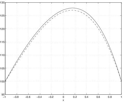
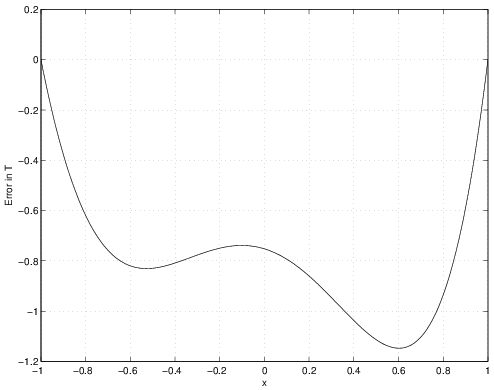
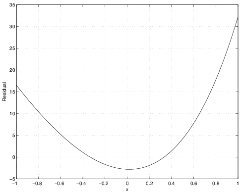
The results using this collocation method are shown in the figures below which include plots of \(\tilde{T}(x)\), the error (i.e., \(\tilde{T}(x)-T(x)\)), and the residual. Note that the residual is exactly zero at the collocation points (i.e., \(x = \pm 1/3\)), though the approximation is not exact at these points (i.e., \(\tilde{T} \neq T\) at \(x = \pm 1/3\)). This is because the residual \(R(\tilde{T},x)\) measures a different thing to the error \(\tilde{T}(x)-T(x)\). Remember, the residual tells us by how much the PDE is not satisfied at a given point, so it relates to the balance between the terms in the PDE (in our case between the term \(\left(k \tilde{T}_ x\right)_ x\) and the heat source term \(f(x)\)). Even if the PDE is satisfied at a particular point (i.e., the residual is zero at that point), the solution might not be exact at that point.