
2.5.3 Finite Volume Method in 2-D
Measurable Outcome 2.1, Measurable Outcome 2.3, Measurable Outcome 2.4
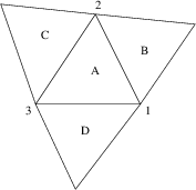
The finite volume discretization can be extended to two-dimensional problems. Suppose the physical domain is divided into a set of triangular control volumes, as shown in Figure 2.15.
Application of Equation 2.1 to control volume A gives,
where \(\Omega _ A\) is the interior and \(\delta \Omega _ A\) is the boundary of control volume A. \(H(U,\vec{n})\) is the flux normal to the face,
As in the one-dimensional case, we define the cell average,
where \(A_ A\) is the area of control volume \(A\). Thus, Equation 2.109 becomes,
In the case of convection, we again assume \(S=0\). Also, we expand the surface integral into the contributions for the three edges,
where \(\vec{n}_{AB}\) is the unit normal pointing from cell A to cell B, and similarly for \(\vec{n}_{AC}\) and \(\vec{n}_{AD}\).
As in one-dimensional case, we assume that the solution everywhere in the control volume is equal to the cell average value. Finally, the flux at each interface is determined by the ‘upwind' value using the velocity component normal to the face. For example, at the interface between cell A and B,
where \(\vec{u}_{AB}\) is the velocity between the control volumes. Thus, when \(\vec{u}_{AB}\cdot \vec{n}_{AB} > 0\), the flux is determined by the state from cell A, i.e. \(U_ A\). Likewise, when \(\vec{u}_{AB}\cdot \vec{n}_{AB} < 0\), the flux is determined by the state from cell B, i.e. \(U_ B\). The velocity, \(\vec{u}_{AB}\) is usually approximated as the velocity at the midpoint of the edge (note: \(\vec{u}\) can be a function of \(\vec{x}\) in two-dimensions even though the velocity is assumed to be divergence free, i.e. \({\partial u}/{\partial x} + {\partial v}/{\partial y} = 0\)). We use the notation \(\hat{H}\) to indicate that the flux is an approximation to the true flux when \(\vec{u}\) is not constant. Thus, the finite volume algorithm prior to time discretization would be given by,
The final step is to integrate in time. As in the one-dimensional case, we might use a forward Euler algorithm which would result in the final fully discrete finite volume method,