2.3.3 Finite Difference Method applied to 1-D Convection
Measurable Outcome 2.2, Measurable Outcome 2.3, Measurable Outcome 2.9, Measurable Outcome 2.10
In this example, we solve 1-D convection,
using a central difference spatial approximation with a forward Euler time integration,
Note: this approximation is the Forward Time-Central Space method from Equation (2.57) with the diffusion terms removed.
Specifically, we will use a constant velocity \(u=1\) and set the initial condition to be a Gaussian disturbance:
We consider the domain \(\Omega =[0.1]\), with periodic boundary conditions. A MATLAB® script that implements this algorithm is:
% This MATLAB script solves the one-dimensional convection
% equation using a finite difference algorithm.  The
% discretization uses central differences in space and forward
% Euler in time.

clear all;
close all;

% Number of points
Nx = 50;
x = linspace(0,1,Nx+1)
dx = 1/Nx;

%velocity
u=1;

% Set final time
tfinal = 10.0;

% Set timestep
dt = 0.001;

% Set initial condition
Uo = 0.75*exp(-((x-0.5)/0.1).^2)';
t = 0;

U = Uo;

% Loop until t > tfinal
while (t < tfinal)
    % Forward Euler Step
    U(2:end) = U(2:end) - dt*u*centraldiff(U(2:end));
    U(1) = U(end); % enforce periodicity

    % Increment time
    t = t + dt;

    % Plot current solution
    clf
    plot(x,Uo,'b*');
    hold on;
    plot(x,U,'*','color',[0 0.5 0]);
    xlabel('x','fontsize',16); ylabel('U','fontsize',16);
    title(sprintf('t = %f\n',t));
    axis([0, 1, -0.5, 1.5]);
    grid on;
    drawnow;
end
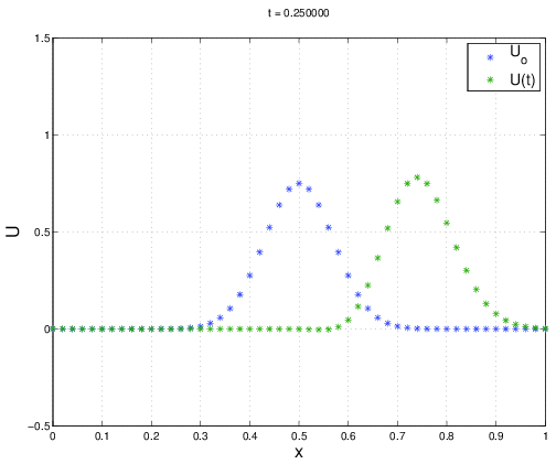
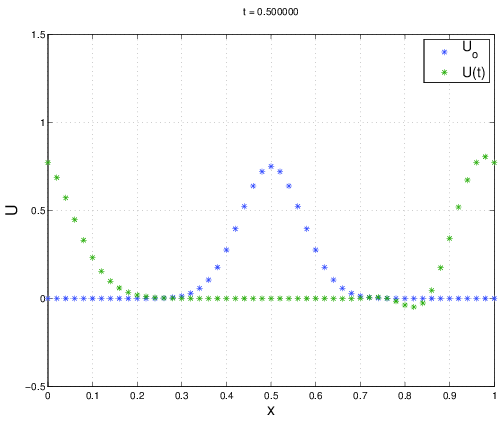
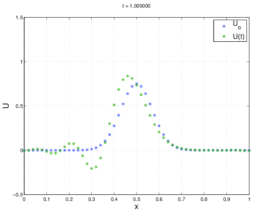
Figures 2.10, 2.11, and 2.12 plot the finite difference solution at times \(t=0.25, t=0.5\) and \(t=1.0\). The exact solution for this problem has \(U(x,t) = U_0(x)\) for any integer time \((t=1,2, \ldots ).\). When the numerical method is run, the Gaussian disturbance is convected across the domain, however small oscillations are observed at \(t=0.5\) which begin to pollute the numerical solution. Eventually, these oscillations grow until the entire solution is contaminated. We will later show that the \(FTCS\) algorithm is unstable for any \(\Delta t\) for pure convection. Thus, what we are observing is an instability that can be predicted through some analysis.