2.7.2 Matrix Stability for Finite Difference Methods
Measurable Outcome 2.2, Measurable Outcome 2.9, Measurable Outcome 2.10, Measurable Outcome 2.11
As we saw in Section 2.3.2, finite difference (or finite volume) approximations can potentially be written in a semi-discrete form as,
While there are some PDE discretization methods that cannot be written in that form, the majority can be. So, we will take the semi-discrete Equation (2.133) as our starting point. Note: the term semi-discrete is used to signify that the PDE has only been discretized in space.
Let \(U(t)\) be the exact solution to the semi-discrete equation. Then, consider perturbation \(e(t)\) to the exact solution such that the perturbed solution, \(V(t)\), is:
The questions that we wish to resolve are: (1) can the perturbation \(e(t)\) grow in time for the semi-discrete problem, and (2) what the stability limits are on the timestep for a chosen time integration method.
First, we substitute \(V(t)\) into Equation (2.133),
Thus, the perturbation must satisfy the homogeneous equation, \(e_ t = A e\). Having studied the behavior of linear system of equations in Section 1.6.2, we know that \(e(t)\) will grow unbounded as \(t \rightarrow \infty\) if any of the real parts of the eigenvalues of \(A\) are positive.
The problem is that determining the eigenvalues of \(A\) can be non-trivial. In fact, for a general problem finding the eigenvalues of \(A\) can be about as hard as solving the specific problem. So, while the matrix stability method is quite general, it can also require a lot of time to perform. Still, the matrix stability method is an indispensible part of the numerical analysis toolkit.
As we saw in the eigenvalue analysis of ODE integration methods, the integration method must be stable for all eigenvalues of the given problem. One manner that we can determine whether the integrator is stable is by plotting the eigenvalues scaled by the timestep in the complex \(\lambda {\Delta t}\) plane and overlaying the stability region for the desired ODE integrator. Then, \({\Delta t}\) can be adjusted to attempt to bring all eigenvalues into the stability region for the desired ODE integrator.
Matrix Stability of FTCS for 1-D convection
Earlier, we used a forward time, central space (FTCS) discretization for 1-d convection,
Since this method is explicit, the matrix \(A\) does not need to be constructed directly, rather Equation (2.138) can be used to find the new values of \(U\) at each point \(i\). However, if we are interested in calculating the eigenvalues to analyze the eigenvalue stability, then the \(A\) matrix is required. The following script does exactly that (i.e. calculates \(A\), determines the eigenvalues of \(A\), and then plots the eigenvalues scaled by \({\Delta t}\) overlayed with the forward Euler stability region). The script can set either the inflow/outflow boundary conditions described in Example 2.3.3, or can set periodic boundary conditions. We will look at the eigenvalues of both cases.
% This MATLAB script calculates the eigenvalues of
% the one-dimensional convection equation discretized by
% finite differences.  The discretization uses central
% differences in space and forward Euler in time.
%
% Periodic bcs are set if periodic_flag == 1.
%
% Otherwise, an inflow (dirichlet) bc is set and at
% the outflow a one-sided (backwards) difference is used.
%

clear all;

periodic_flag = 1;

% Set-up grid
xL = -4;
xR =  4;
Nx = 21; % number of points
x = linspace(xL,xR,Nx);

% Calculate cell size in control volumes (assumed equal)
dx = x(2) - x(1);

% Set velocity
u = 1;

% Set timestep
CFL = 1;
dt = CFL*dx/abs(u);

% Set bc state at left (assumes u>0)
UL = exp(-xL^2);

% Allocate matrix to hold stiffness matrix (A).
%
A = zeros(Nx-1,Nx-1);

% Construct A except for first and last row
for i = 2:Nx-2,
  A(i,i-1) =  u/(2*dx);
  A(i,i+1) = -u/(2*dx);
end

if (periodic_flag == 1), % Periodic bcs

  A(1   ,2   ) = -u/(2*dx);
  A(1   ,Nx-1) =  u/(2*dx);
  A(Nx-1,1   ) = -u/(2*dx);
  A(Nx-1,Nx-2) =  u/(2*dx);

else % non-periodic bc's

  % At the first interior node, the i-1 value is known (UL).
  % So, only the i+1 location needs to be set in A.
  A(1,2) = -u/(2*dx);

  % Outflow boundary uses backward difference
  A(Nx-1,Nx-2) =  u/dx;
  A(Nx-1,Nx-1) = -u/dx;

end

% Calculate eigenvalues of A
lambda = eig(A);

% Plot lambda*dt
plot(lambda*dt,'*');
xlabel('Real \lambda\Delta t');
ylabel('Imag \lambda\Delta t');

% Overlay Forward Euler stability region
th = linspace(0,2*pi,101);
hold on;
plot(-1 + sin(th),cos(th));
hold off;
axis('equal');
grid on;
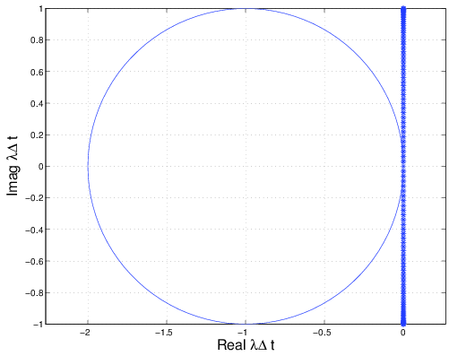
Figures 2.21 and 2.22 show plots of \(\lambda {\Delta t}\) for a CFL set to one. Recall that for this one-dimensional problem, the CFL number was defined as,
In the inflow/outflow boundary condition case (shown in Figure 2.21) the eigenvalues lay slightly inside the negative real half-plane. As they move away from the origin, they approach the imaginary axis at \(\pm i\). The periodic boundary conditions give purely imaginary eigenvalues but these also approach \(\pm i\) as the move away from the origin. Note that the periodic boundary conditions actually give a zero eigenvalue so that the matrix \(A\) is actually singular (Why is this?). Regardless what we see is that for a \(\mathrm{CFL} = 1\), some \(\lambda {\Delta t}\) exist which are outside of the forward Euler stability region. We could try to lower the timestep to bring all of the \(\lambda {\Delta t}\) into the stability region, however that will prove to be practically impossible since the extreme eigenvalues approach \(\pm \alpha i\) (i.e. they are purely imaginary). Thus, no finite value of \({\Delta t}\) exists for which these eigenvalues can be brought inside the circular stability region of the forward Euler method (i.e. the FTCS is unstable for convection).
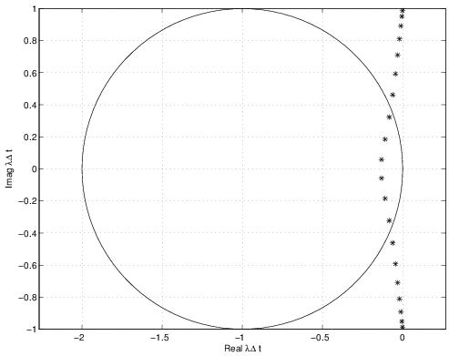
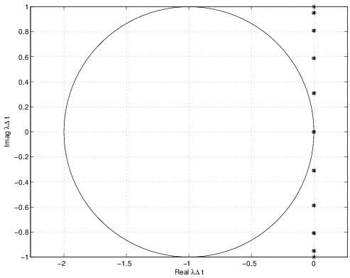
We may also be interested in what happens to the eigenvalue spectrum of \(A\) when we change \(\Delta x\) keeping the CFL constant. Figures 2.23 and 2.24 plot the eigenvalue spectrum for both periodic and Dirichlet boundary conditions refining \(\Delta x\) by a factor of 10. For the periodic BC case, again we see purely imaginary eigenvalues approaching \(\pm i\) (though, of course, we have more eigenvalues as \(A\) is now a larger system). For the Dirichlet case, the eigenvalues again lie slightly inside the negative real half-plane, though in this case closer to the imaginary axis than for the coarser system. In fact, the eigenvalues of the Dirichlet problem approach those of the periodic problem in the limit as \(\Delta x \to 0\).