
1.6.3 Eigenvalue Stability for a Linear ODE
Measurable Outcome 1.2, Measurable Outcome 1.3, Measurable Outcome 1.6, Measurable Outcome 1.9, Measurable Outcome 1.18
As we have seen, while numerical methods can be convergent, they can still exhibit instabilities as \(n\) increases for finite \({\Delta t}\). For example, when applying the midpoint method to either the ice particle problem in Section 1.2.4 or the simpler model problem in Example 1.66, instabilities were seen in both cases as \(n\) increased. Similarly, for the nonlinear pendulum problem in Example 1.86, the forward Euler method had a growing amplitude again indicating an instability. The key to understanding these results is to analyze the stability for finite \({\Delta t}\). This analysis is different than the stability analysis we performed in Section 1.5.2 since that analysis was for the limit of \({\Delta t}\rightarrow 0\).
Suppose we are interested in solving the linear ODE,
Consider the Forward Euler method applied to this problem,
Similar to the zero stability analysis, we will assume that the solution has the following form,
where \(g\) is the amplification factor (and the superscript \(n\) acting on \(g\) is again raising to a power). As in the zero stability analysis, we wish to determine under what conditions \(|g| > 1\) since this would mean that \(v^ n\) will grow unbounded as \(n \rightarrow \infty\). Substituting Equation 1.101 into Equation 1.100 gives,
Thus, the only non-zero root of this equation gives,
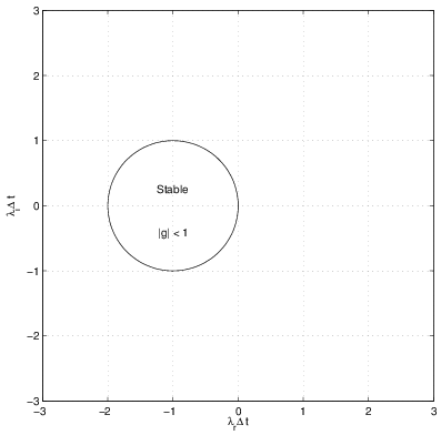
which is the amplification factor for the forward Euler method. Now, we must determine what values of \(\lambda {\Delta t}\) lead to instability (or stability). A simple way to do this for multi-step methods is to solve for the stability boundary for which \(|g| = 1\). To do this, let \(g = e^{i\theta }\) (since \(|e^{i\theta }| = 1\)) where \(\theta = [0,2\pi ]\). Making this substitution into the amplification factor,
Thus, the stability boundary for the forward Euler method lies on a circle of radius one centered at -1 along the real axis and is shown in Figure 1.10.
For a given problem, i.e. with a given \(\lambda\), the timestep must be chosen so that the algorithm remains stable for \(n \rightarrow \infty\). Let's consider some examples.
Example
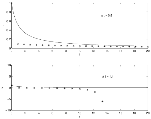
Let's return to the previous example, \(u_ t = -u^2\) with \(u(0) = 1\). To determine the timestep restrictions, we must estimate the eigenvalue for this problem. Linearizing this problem about a known state gives the eigenvalue as \(\lambda = {\partial f}/{\partial u} = -2u\). Since the solution will decay from the initial condition (since \(u_ t < 0\) because \(-u^2 < 0\)), the largest magnitude of the eigenvalue occurs at the initial condition when \(u(0) = 1\) and thus, \(\lambda = -2\). Since this eigenvalue is a negative real number, the maximum \({\Delta t}\) will occur at the maximum extent of the stability region along the negative real axis. Since this occurs when \(\lambda {\Delta t}= -2\), this implies that \({\Delta t}< 1\). To test the validity of this analysis, the forward Euler method was run for \({\Delta t}= 0.9\) and \({\Delta t}= 1.1\). The results are shown in Figure 1.11 which are stable for \({\Delta t}= 0.9\) but are unstable for \({\Delta t}= 1.1\).
Pendulum Example
Next, let's consider the application of the forward Euler method to the pendulum problem. For this case, the linearization produces a matrix,
The eigenvalues can be found from the roots of the determinant of \({\partial f}/{\partial u} - \lambda I\):
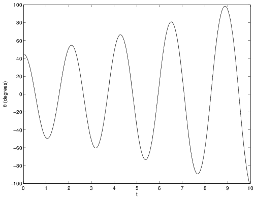
Thus, we see that the eigenvalues will always be imaginary for this problem. As a result, since the forward Euler stability region does not contain any part of the imaginary axis (except the origin), no finite timestep exists which will be stable. This explains why the amplitude increases for the pendulum simulations in Figure 1.8.