1.9 Runge-Kutta Methods

1.9.3 Stability Regions

Measurable Outcome 1.16, Measurable Outcome 1.18, Measurable Outcome 1.19

The eigenvalue stability regions for Runge-Kutta methods can be found using essentially the same approach as for multi-step methods. Specifically, we consider a linear problem in which \(f = \lambda u\) where \(\lambda\) is a constant. Then, we determine the amplification factor \(g = g(\lambda {\Delta t})\). For example, let's look at the modified Euler method,

	\(\displaystyle a\)	\(\displaystyle =\)	\(\displaystyle {\Delta t}\lambda v^ n\)		(1.150)
	\(\displaystyle b\)	\(\displaystyle =\)	\(\displaystyle {\Delta t}\lambda \left(v^ n + {\Delta t}\lambda v^ n/2\right)\)		(1.151)
	\(\displaystyle v^{n+1}\)	\(\displaystyle =\)	\(\displaystyle v^ n + {\Delta t}\lambda \left(v^ n + {\Delta t}\lambda v^ n/2\right)\)		(1.152)
	\(\displaystyle v^{n+1}\)	\(\displaystyle =\)	\(\displaystyle \left[1 + {\Delta t}\lambda + \frac{1}{2}({\Delta t}\lambda )^2 \right]v^ n\)		(1.153)
	\(\displaystyle \Rightarrow g\)	\(\displaystyle =\)	\(\displaystyle 1 + \lambda {\Delta t}+ \frac{1}{2}(\lambda {\Delta t})^2\)		(1.154)

A similar derivation for the four-stage scheme shows that,

\[g = 1 + \lambda {\Delta t}+ \frac{1}{2}(\lambda {\Delta t})^2 + \frac{1}{6}(\lambda {\Delta t})^3 + \frac{1}{24}(\lambda {\Delta t})^4.\]

(1.155)

When analyzing multi-step methods, the next step would be to determine the locations in the \(\lambda {\Delta t}\)-plane of the stability boundary (i.e. where \(|g|=1\)). This however is not easy for Runge-Kutta methods and would require the solution of a higher-order polynomial for the roots. Instead, the most common approach is to simply rely on a contour plotter in which the \(\lambda {\Delta t}\)-plane is discretized into a finite set of points and \(|g|\) is evaluated at these points. Then, the \(|g|=1\) contour can be plotted. The following is the MATLAB^® code which produces the stability region for the second-order Runge-Kutta methods (note: \(g(\lambda {\Delta t})\) is the same for both second-order methods):

% Specify x range and number of points
x0 = -3;
x1 =  3;
Nx = 301;

% Specify y range and number of points
y0 = -3;
y1 =  3;
Ny = 301;

% Construct mesh
xv    = linspace(x0,x1,Nx);
yv    = linspace(y0,y1,Ny);
[x,y] = meshgrid(xv,yv);

% Calculate z
z = x + i*y;

% 2nd order Runge-Kutta growth factor
g = 1 + z + 0.5*z.^2;

% Calculate magnitude of g
gmag = abs(g);

% Plot contours of gmag
contour(x,y,gmag,[1 1],'k-');
axis([x0,x1,y0,y1]);
axis('square');
xlabel('Real \lambda\Delta t');
ylabel('Imag \lambda\Delta t');
grid on;

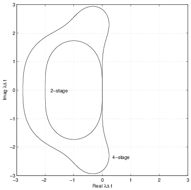
The plots of the stability regions for the second and fourth-order Runge-Kutta algorithms is shown in Figure 1.25. These stability regions are larger than those of multi-step methods. In particular, the stability regions of the multi-stage schemes grow with increasing accuracy while the stability regions of multi-step methods decrease with increasing accuracy.