
1.3.2 Local Truncation Error
Global error measures the difference between the computed solution at a given time and the true solution of the initial value problem that we are trying to solve. Local error is the error made in one step of the numerical method. While we are generally interested in obtaining small global errors, local errors are the errors over which we have direct control. Both global and local accuracy are related to the behavior of the error as \({\Delta t}\rightarrow 0\). Convergence is related to global accuracy; for local accuracy we will see in 1.5.1 an important concept known as consistency.
If we can quantify how much the error changes in a single timestep, then we will have an indication of how much the error could change over a series of timesteps. Specifically, let's write the solution error, \(e\), at \(t=T\) as a sum of the change in error at each timestep,
where \(\Delta e^ n\) is the change in the error from iteration \(n-1\) to \(n\) (i.e. the local error). Suppose the local error is \(O({\Delta t}^{p+1})\), then the global error might be expected to behave as,
Thus, the global error would decrease with \({\Delta t}\) by one order less than the local error because the local errors sum for \(T/{\Delta t}\) timesteps. However, we must be careful because the local errors do not have to sum this way, particularly if the numerical method is not stable. We will see in the next lecture that if a numerical method is both consistent and stable, this will be enough to guarantee convergence. For now, we concentrate on quantifying the local accuracy and leave the discussion of consistency and stability for another lecture.
The local error (usually called the local truncation error) is the difference between the approximate solution at step \(n+1\) and the solution at \(t^{n+1}\) of the ODE that passes through the previous computed point \(v^ n\). The local error can be evaluated by considering the difference between the approximate solution at step \(n+1\) computed using the exact solution for the required data and the exact solution at \(t^{n+1}\).
Example: Local error of the forward Euler method
Let's consider the forward Euler method as an example. Recall, the forward Euler method is,
Thus, for the forward Euler method, \(v^{n+1} = v^{n+1}(v^ n,{\Delta t},t^ n)\). Then, if we substitute the exact solution into the right-hand side, we find,
Recall our notation that \(u\) is the exact solution; in this discussion we use the superscript notation \(u^ n = u(n{\Delta t})\) realizing that \(u = u(t)\). Therefore the equation above gives the value of \(v^{n+1}\) that would be computed if the exact solution were available at time \(t^ n\). The local truncation error for the forward Euler method is then,
Substitution gives,
The local order of accuracy is then found using a Taylor series expansion about \(t = t^ n\). Recall that \(f(u^ n,t^ n) = u_ t(t^ n)\) and
Substitution gives the local truncation error as,
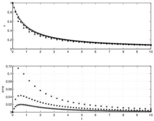
Thus, the leading term of the local truncation error for the forward Euler method is \(-\frac{1}{2}{\Delta t}^2 u_{tt}(t^ n) = O({\Delta t}^2)\). Based on our previous argument, we expect that the global accuracy of the forward Euler method should be \(O({\Delta t})\) (i.e. first order accuracy). This was in fact observed in Example 1.5.