
1.4.3 Rate of Convergence (Global Order of Accuracy)
In addition to knowing whether a numerical method will converge, we are also interested to know at what rate will it converge. The rate of convergence is known as the global order of accuracy and describes the decrease in error \(\max _{n \in \{ 0,1,\ldots ,T/ {\Delta t}\} }|v^ n-u^ n|\) one can expect for a given decrease in time step \({\Delta t}\) in the limit \({\Delta t}\to 0\).
Definition of Global Accuracy
A method has a global order of accuracy of \(p\) if,
for any \(f(u,t)\) that has \(p\) continuous derivatives (i.e. up to and including \({\partial ^ p f}/{\partial t^ p}\) and \({\partial ^ p f}/{\partial u^ p}\)).
Thus, methods with higher \(p\) will converge to \(u(t)\) more rapidly than those methods with lower \(p\). This is the second time we've come across the \(\mathcal{O}()\) notation. Recall that this means that the terms on the right side of the expression \(\max _{n \in \{ 0,1, \ldots ,T/{\Delta t}\} }|v^ n-u^ n|\leq \mathcal{O}({\Delta t}^ p)\) can be accurately approximated by \(c{\Delta t}^ p\) for some constant \(c\) in the limit \({\Delta t}\to 0\).
That is, terms of the form \({\Delta t}^ q\) for \(q>p\) can be safely ignored since they are much smaller in magnitude than \({\Delta t}^ p\) in the limit \({\Delta t}\to 0\). Let's consider the meaning of this statement in more depth. If a method has global order of accuracy p, in the limit \({\Delta t}\to 0\), if we shrink the time step by a factor of two, we can expect the worst case error in the approximation to decrease by a factor of \(2^ p\). Therefore, the higher the global order of accuracy, the faster the convergence rate of the numerical method. For a first-order accurate method (\(p=1\)), we expect that decreasing the time step by a factor of two (cutting it in half) would result in the halving of the worst case error. Likewise, for a second-order accurate method (\(p=2\)), decreasing the time step by a factor of two should lead to the quartering of the worst case error. (It is important to remember that these statements only hold in the limit \({\Delta t}\to 0\). You will find that these results hold approximately for small \({\Delta t}\), but as you increase \({\Delta t}\) you will likely not observe this behavior.) We will now demonstrate this behavior numerically for the forward Euler method.
Forward Euler and Midpoint accuracy on example problem
To demonstrate the ideas of global accuracy, we will consider an ODE with
and an initial condition of \(u(0) = 1\). The solution to this ODE is \(u = (1+t)^{-1}\). Now, let us apply the forward Euler method to solving this problem for \(t=0\) to \(10\). The approximate solutions for a range of \({\Delta t}\) are shown Figure 1.5 along with the exact solution.
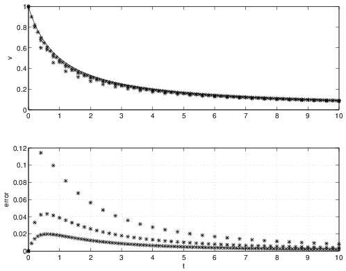
The forward Euler solutions are clearly approaching the exact solution as \({\Delta t}\) decreases. Furthermore, the error appears to be decreasing by approximately a factor of 2 for every factor of 2 decrease in \({\Delta t}\). For example, if we look at \(t=4\), the error is seen to be \(0.028\), \(0.013\), and \(0.0065\) for \({\Delta t}= 0.4\), \(0.2\), and \(0.1\), respectively.
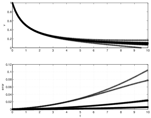
Now, let's apply the midpoint method on the problem from Equation 1.66. Similar to the results observed using the midpoint rule for the ice falling problem the midpoint method shows an oscillatory behavior (this may be a little hard to see because of scale of the figure, but the midpoint results are basically oscillated about the exact solution, with the oscillations reducing for the smaller timesteps). Note that the timesteps used in these results are a factor of 10 smaller than those used with the forward Euler method. Since the midpoint and the forward Euler method require essentially the same work per timestep, the midpoint results took about a factor of 10 more work than the forward Euler method for this problem. Another interesting aspect of these results is that the error is actually increasing as \(t\) increases (in the forward Euler results in Figure 1.5, the error decreased as \(t\) increased). Regardless, the method does appear convergent since as the timestep decreases, so are the errors. In fact, it appears that the errors are decreasing by a factor of 4 for a factor of 2 decrease in \({\Delta t}\). For example, if we look at \(t=4\), the error (averaged to remove the oscillations) is seen to be approximately \(0.02\), \(0.005\), and \(0.00125\) for \({\Delta t}= 0.04\), \(0.02\), and \(0.01\), respectively.
Exercise 1 Use the relevent plots above to determine the global order of accuracy for the forward Euler method.
Exercise 2 Use the plots above to determine the global order of accuracy for the Midpoint method.