
Functions define a small world of variables that are isolated from the rest of the "workspace". This is mostly a good thing, though you may find it limiting at times. It is important to realize that a function can call itself, and even then the variables inside the called function cannot interact directly with those of the calling workspace. Here is an example to show this:
functiontriangle(n) n if n > 1 triangle(n-1) end n
This is a function with no output, that calls itself. Calling it from the command-line gives:
>> triangle(4) n = 4 n = 3 n = 2 n = 1 n = 1 n = 2 n = 3 n = 4Exercise 14: Write a function that recursively (a function that calls itself is called recursive) calculates the Fibonacci numbers:
$$ F_1=1, \qquad F_2=1, \qquad F_{n+2}=F_{n}+F_{n+1} $$
Try it out for small value of n (it will not work for large ones). (The resulting sequence is 1, 1, 2, 3, 5, 8, 13, 21, 34, 55,....)
User-defined functions are useful in providing structure to your code. When writing code try to think in terms of functions. Separate the big task into smaller ones and define them in terms of input and output. Your main code should then be easier to read as it will consist of calls to the functions, each of which has a clearly defined task. Notice that in a function file, one can define more than one function. Simply start a new line with the keyword function and continue as before. This function will only be directly callable from within the file (since the name of the file matches a different function) though there are tricks by which one can still provide access to such "hidden" functions (too advanced for this course).
For guided practice and further exploration of scripted functions, watch Video Lecture 5: Scripts and Functions.
Here's an example of a function that calculates and plots the solution to the Van-der-Pol oscillator (must be saved into a file called VDPDemo.m):
functionVDPDemo(mu) % solve an ODE using Runge-Kutta 4/5: [t,X]=ode45(@dXdt,[0,100],[0;1]); % plot the resulting phase plane trajectory: plot(X(:,1),X(:,2)) % Here we define the derivative function. % By nesting this function inside the main one, we get access to the % variable mu, defined in the outer function function dX=dXdt(t,X) x=X(1); v=X(2); dx=v; dv=-x+mu*(1-x^2)*v; dX=[dx;dv]; end % of dXdtg end % of VDPDemo % Were the function dXdt defined here, (after the end keyword that closes % the VDPDemo function) the variable mu would be undefined and the code % would not run.
We can run this function by calling it with the value for mu from the command prompt:
>> VDPDemo(2)which results in the figure:
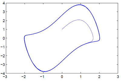
Plotting the solution to the Van-der-Pol oscillator.
Exercise 15: Run the Van-der-Pol oscillator several times with various input values. Observe the change in shape.
Change the code for the Van-der-Pol oscillator:
- Add a green marker at the beginning of the trajectory
- Add a red marker at the end of the trajectory
- Plot an approximation of the "limit cycle" in black
-
(Bonus) find out what the period of the limit cycle is, modify the function so that it returns this value, write an additional function or script that calls
VDPDemofor many values ofmuand plots the dependence of the period onmu. Perhaps, to find the period of the limit cycle, you can write a function that accepts an approximation to the period of the limit cycle and returns a positive number if it's too big and a negative number when it's too small. you can then use this function with a secant method root finder, to find quickly the period of the limit cycle.
(Hint 1: Read the helpfile for plot carefully to understand how to change the defaults) (Hint 2: Remember that to plot several plots on the same figure without erasing the previous figure you need to issue a hold on command.)
Homework 3. Debug this code. Put a break-point on the first line in the inner function and run the code (with input 2 for example). Step over ode45 and see how you can see the values of variables by "hovering" the mouse pointer over the variable in the editor. This only works if the variable can be "seen" from the current scope. Click "step" a few times to see the code advancing.
Now terminate this execution.
Change the code so that the function dXdt is defined outside the main function (by moving one end placement). Debug again and notice how the variable mu is no longer visible inside the function dXdt. At what point does the code fail?
For guided practice and further exploration of debugging, watch Video Lecture 6: Debugging.