
Topics
- Games with homogeneous externalities
- Games with local network effects
Recall
Congestion games had simple sets of payoffs but complicated network structure. There are games that have complicated payoffs with simple network structure.
Homogeneous Externalities
In classical economics, the demand curve is assumed decreasing and the supply curve increasing. The existence of network effects may create a weird shape of the demand curve.
- N = [0, 1] continuum of players
- Si = {buy, not buy}
-
ui(Si, S-i) = ui(Si, x) =
vix — p if Si = buy
0 if Si= not buy - vi ~ F([0, 1])
- p > 0
- Where x is how many buy, vi is its value, and p is price.
Example: Office suites, SNS, etc.
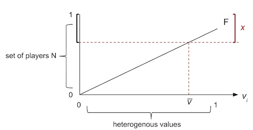
- x = 1 — F(v̅) where v̅ is the lowest value of agents who buy.
Claim: If agent with vi = v̅ is better off buying, then any agent with vj > v̅ is also better off buying.
Corollary: We may assume without loss of generality that x (those who buy) have the highest values in equilibrium/socially optimal outcome.
- Socially optimal outcome
- Social welfare = v̅∫1[v(1 — F(v̅)) — p] dF(v)
- Maximizing this with respect to v̅ yields the social best.
- Nash equilibrum
- Pooling equilibrum:
If no one has the good (x = 0) then no one has incentive to buy ( vi * 0 — p < 0). Therefore, x* = 0 is an equilibrium. - Separating equilibrium:
If someone buys (x > 0), then there exists the lowest type v̅ who buys. His incentive must balance v̅x — p = 0.
- Pooling equilibrum:
Note that everyone's strategy is summarized by x. So consider the aggregate best response function BR(x) = x̂. With v̅x — p = 0 and x = 1 — F(v̅), we find:
- BR(x) = 1 — F(p/x).
- Its fixed point x* is an equilibrium.
Local Network Effects
Some games have both complicated payoff structure and complicated network structure.
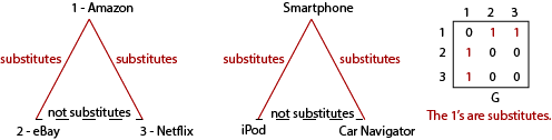
- N = {1, 2, 3}.
- Si = ℝ+ = [0, ∞).
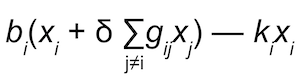
-
ui(xi, x-i, δ, G) =
i's best response satisfies
![]()
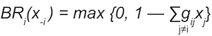
- BR(x) = max { 𝟘, 𝟙 — δG𝕏}